Solving QUBO/Ising Problems via Unit-Disk Graphs on Neutral Atom Quantum Computer

Install dependencies

# !pip install bloqade-analog

Formulating the Problem Hamiltonian

In the following part, we demonstrate how to use the Jijmodleing to fomulate the problem Hamiltonian.

import numpy as np
import jijmodeling as jm


def QUBO_problem():
    # --- placeholders ---
    V = jm.Placeholder("V")
    E = jm.Placeholder("E", ndim=2)
    U = jm.Placeholder("U", ndim=2)

    n = jm.BinaryVar("n", shape=(V,))
    e = jm.Element("e", belong_to=E)

    # --- build problem ---
    problem = jm.Problem("QUBO_Hamiltonian")

    quadratic_term = jm.sum(e, U[e[0], e[1]] * n[e[0]] * n[e[1]])
    problem += quadratic_term
    return problem


problem = QUBO_problem()
problem

\[\begin{split}\begin{array}{cccc}\text{Problem:} & \text{QUBO\_Hamiltonian} & & \\& & \min \quad \displaystyle \sum_{e \in E} U_{e_{0}, e_{1}} \cdot n_{e_{0}} \cdot n_{e_{1}} & \\\text{{where}} & & & \\& n & 1\text{-dim binary variable}\\\end{array}\end{split}\]

import numpy as np

quad = {
    (0, 0): -1.2,
    (1, 1): -3.2,
    (2, 2): -1.2,
    (0, 1): 4.0,
    (0, 2): -2.0,
    (1, 2): 3.2,
}

V_val = 3
E_val = np.array(list(quad.keys()), dtype=int)
U_val = np.zeros((V_val, V_val))
for (i, j), Jij in quad.items():
    U_val[i, j] = U_val[j, i] = Jij

instance = {
    "V": V_val,
    "E": E_val,
    "U": U_val,
}

compiled_instance = jm.Interpreter(instance).eval_problem(problem)

Converting the Problem with qamomile

Once, we obtain the compiled_instance, the QuantumConverter can convert it to the IsingModel class.

from qamomile.core.converters.qaoa import QAOAConverter

udm_converter = QAOAConverter(compiled_instance)
ising_model = udm_converter.ising_encode()
ising_model

IsingModel(quad={(0, 1): 1.0, (0, 2): -0.5, (1, 2): 0.8}, linear={0: 0.09999999999999998, 1: -0.19999999999999996, 2: 0.30000000000000004}, constant=-1.5000000000000002, index_map=None)

Unit-Disk Mapping with qamomile

Performing the Mapping: UnitDiskGraph Class

The UnitDiskGraph class handles the conversion from an IsingModel to the UDG representation.

from qamomile.udm import Ising_UnitDiskGraph

udg = Ising_UnitDiskGraph(ising_model)

print(f"Converted to Unit Disk Graph:")
print(f"- {len(udg.nodes)} nodes in the grid graph")
print(f"- {len(udg.pins)} pins (nodes corresponding to original variables)")

Overwriting delta from 2.7 to 1.5
Converted to Unit Disk Graph:
- 26 nodes in the grid graph
- 3 pins (nodes corresponding to original variables)

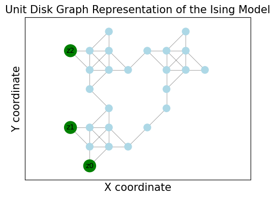
Visualizing the UDG

We can visualize the resulting UDG structure using networkx and matplotlib. The UnitDiskGraph object provides access to the underlying graph structure. This visualization helps understand how the abstract Ising problem is physically laid out using the UDM gadgets.

import matplotlib.pyplot as plt
import networkx as nx

G_vis = udg.networkx_graph
pos = nx.get_node_attributes(G_vis, "pos")
pins = udg.pins
plt.figure(figsize=(5, 4))

# Highlight pins (original variables)
node_colors = ["Green" if i in pins else "lightblue" for i in G_vis.nodes()]
node_sizes = [300 if i in pins else 100 for i in G_vis.nodes()]

nx.draw_networkx_nodes(G_vis, pos, node_color=node_colors, node_size=node_sizes)
nx.draw_networkx_edges(G_vis, pos, width=0.5, alpha=0.5)

# Label the pins with their original variable index
pin_labels = {pin: f"z{i}" for i, pin in enumerate(pins)}  # Use z_i for Ising spins
nx.draw_networkx_labels(G_vis, pos, labels=pin_labels, font_size=10)

plt.title("Unit Disk Graph Representation of the Ising Model", fontsize=15)
plt.xlabel("X coordinate", fontsize=15)
plt.ylabel("Y coordinate", fontsize=15)
plt.axis("equal")  # Ensure aspect ratio is maintained
plt.tight_layout()
plt.show()

Solving MWIS-UDG with bloqade-analog

Now that we have mapped the original Ising problem to an MWIS problem on a Unit-Disk Graph, we can leverage the native capabilities of neutral atom quantum computers to find the solution.

Implementation with bloqade-analog

bloqade-analog is a Python library for simulating analog neutral atom quantum computations, particularly suited for adiabatic protocols like the one described above. The bloqade_example.py script shows how to use it with our UDG mapping.

Steps:

1. Prepare Inputs:

   • Get atom locations from the UnitDiskGraph object (udg.nodes). These locations need to be scaled to physical units (e.g., micrometers) appropriate for typical blockade radii.

   • Get node weights (udg.nodes[i].weight). These weights are typically normalized.

   • Define the pulse parameters: maximum Rabi frequency Omega_max, maximum detuning delta_max, and total evolution time t_max.

import numpy as np
import math

LOCATION_SCALE = 5.0  # Adjust based on desired blockade radius and hardware

locations = udg.qubo_result.qubo_grid_to_locations(LOCATION_SCALE)
weights = udg.qubo_result.qubo_result_to_weights()

print(f"Node weights: {weights}")
print(f"Node locations: {locations}")

Node weights: [1.3, 1.8, 1.6, 5.0, 7.0, 3.0, 6.5, 5.5, 7.0, 5.0, 3.0, 5.5, 6.5, 1.4, 3.0, 3.0, 3.0, 3.0, 3.0, 3.0, 5.2, 6.8, 6.8, 5.2, 1.7, 1.2]
Node locations: [(0.0, 10.0), (0.0, 30.0), (5.0, 0.0), (5.0, 5.0), (5.0, 10.0), (5.0, 20.0), (5.0, 25.0), (5.0, 30.0), (10.0, 5.0), (10.0, 10.0), (10.0, 15.0), (10.0, 25.0), (10.0, 30.0), (10.0, 35.0), (15.0, 5.0), (15.0, 25.0), (20.0, 10.0), (20.0, 30.0), (25.0, 15.0), (25.0, 20.0), (25.0, 25.0), (25.0, 30.0), (30.0, 25.0), (30.0, 30.0), (30.0, 35.0), (35.0, 25.0)]

2. Define the Program: Use bloqade.analog to define the atom geometry and pulse sequence.

from bloqade.analog import start


def solve_ising_bloqade(locations, weights, delta_max=60.0, Omega_max=15.0, t_max=4.0):
    locations_array = np.array(locations)
    centroid = locations_array.mean(axis=0)
    centered_locations = locations_array - centroid
    locations = list(map(tuple, centered_locations))

    lw = len(weights)
    weights_norm = [x / max(weights) for x in weights]

    def sine_waveform(t):
        return Omega_max * math.sin(math.pi * t / t_max) ** 2

    def linear_detune_waveform(t):
        return delta_max * (2 * t / t_max - 1)

    program = (
        start.add_position(locations)
        .rydberg.detuning.scale(weights_norm)
        .fn(linear_detune_waveform, t_max)
        .amplitude.uniform.fn(sine_waveform, t_max)
    )

    return program


program = solve_ising_bloqade(locations, weights)

3. Run the Simulation: Execute the program using Bloqade’s emulator.

blockade_radius = (
    LOCATION_SCALE * 1.5
)  # blockade radius is set to cover the diagonoal node (1: sqrt(2))
emu_results = program.bloqade.python().run(
    shots=10000, solver_name="dop853", blockade_radius=blockade_radius
)

report = emu_results.report()
counts = report.counts()[0]

sorted_counts = {
    k: v for k, v in sorted(counts.items(), key=lambda item: item[1], reverse=True)
}

print("\nBloqade Simulation Results (Top 5):")
for i, (bitstring, count) in enumerate(list(sorted_counts.items())[:5]):
    print(f" {i+1}. Bitstring: {bitstring} (Count: {count})")

Bloqade Simulation Results (Top 5):
 1. Bitstring: 10010011111101011001110101 (Count: 703)
 2. Bitstring: 10010011111101011101101110 (Count: 298)
 3. Bitstring: 11010101111110011001110101 (Count: 291)
 4. Bitstring: 11010101111110001101101110 (Count: 286)
 5. Bitstring: 10110011111101011001110101 (Count: 285)

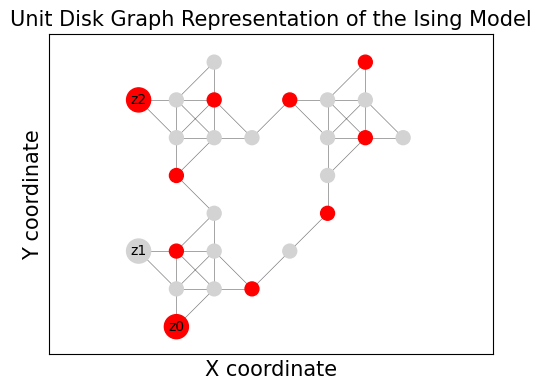
Visualizing the result from Bloqade’s emulator.

We can visualize the result from Bloqade’s emulator. The red node shows the mapping of the Bitstring.

import matplotlib.pyplot as plt
import networkx as nx

G_vis = udg.networkx_graph
pos = nx.get_node_attributes(G_vis, "pos")

plt.figure(figsize=(5, 4))

bitstr = list(sorted_counts.items())[:2][0][0]

# Color and size nodes based on bit value
node_colors = ["red" if b == "0" else "lightgray" for b in bitstr]
node_sizes = [300 if i in pins else 100 for i in G_vis.nodes()]

nx.draw_networkx_nodes(G_vis, pos, node_color=node_colors, node_size=node_sizes)
nx.draw_networkx_edges(G_vis, pos, width=0.5, alpha=0.5)

# Label the pins with their original variable index
pin_labels = {pin: f"z{i}" for i, pin in enumerate(pins)}  # Use z_i for Ising spins
nx.draw_networkx_labels(G_vis, pos, labels=pin_labels, font_size=10)

plt.title("Unit Disk Graph Representation of the Ising Model", fontsize=15)
plt.xlabel("X coordinate", fontsize=15)
plt.ylabel("Y coordinate", fontsize=15)
plt.axis("equal")  # Ensure aspect ratio is maintained
plt.tight_layout()
plt.show()

Converting the Bloqade’s emulator result to sampleset result.

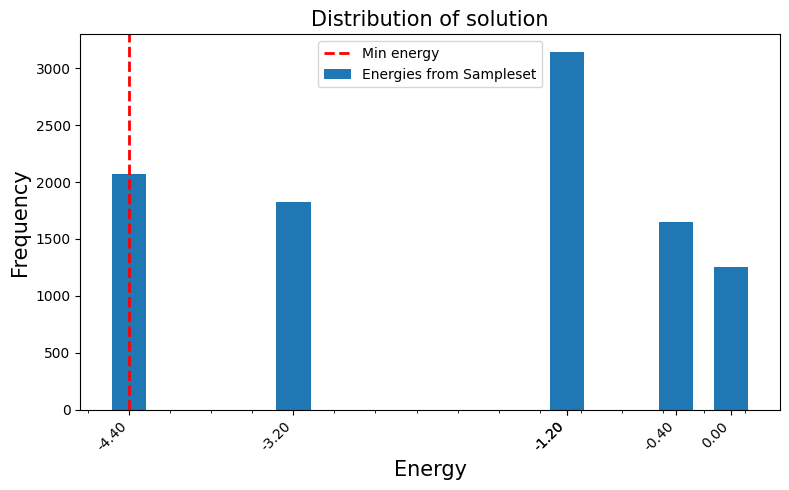
From the emulator result obtained earlier, we can transfer them to a sampleset by udm_converter.decode. The sampleset can examine the distribution of the objective function values.

from qamomile.udm.transpiler import UDMTranspiler

transpiler = UDMTranspiler(udg, V_val)
sampleset = udm_converter.decode(transpiler, counts)

Check the lowest solution

sampleset.lowest()

[Sample(run_id="0f45e0fa-bfd0-408f-856f-d76ad80e5f78", num_occurrences=2181, run_info={}, var_values={"n": SparseVarValues(name="n", values={(0,): 1, (2,): 1}, shape=(3,), var_type=VarType.CONTINUOUS)}, eval=EvaluationResult(objective=-4.4, constraints={}, penalties={}))]

Check the classcical method

import numpy as np
from itertools import product

Q = np.array([[-1.2, 4.0, -2.0], [4.0, -3.2, 3.2], [-2.0, 3.2, -1.2]])


def Solve_Q(Q: np.ndarray, x: np.ndarray) -> float:
    E = np.dot(np.diag(Q), x)
    n = len(x)
    for i in range(n):
        for j in range(i + 1, n):
            E += Q[i, j] * x[i] * x[j]
    return E


energies = {}
for bits in product([0, 1], repeat=3):
    x = np.array(bits)
    energy = Solve_Q(Q, x)
    energies[bits] = energy
min_config, min_energy = min(energies.items(), key=lambda item: item[1])
print("min_config: ", min_config)
print("min_energy: ", min_energy)

min_config:  (1, 0, 1)
min_energy:  -4.4

import numpy as np
import matplotlib.pyplot as plt
from matplotlib.ticker import MultipleLocator, AutoMinorLocator, FormatStrFormatter

plot_data = {}
for sample in sampleset:
    if sample.eval.objective in plot_data:
        plot_data[sample.eval.objective] += sample.num_occurrences
    else:
        plot_data[sample.eval.objective] = sample.num_occurrences

energies = sorted(plot_data.keys())
freqs = [plot_data[e] for e in energies]
plt.figure(figsize=(8, 5))
plt.bar(energies, freqs, width=0.25, label="Energies from Sampleset")

ax = plt.gca()
ax.set_xticks(energies)
ax.set_xticklabels([f"{e:.2f}" for e in energies], rotation=45, ha="right")
ax.axvline(min_energy, color="red", linestyle="--", linewidth=2, label="Min energy")

ax.xaxis.set_minor_locator(AutoMinorLocator(4))

plt.title("Distribution of solution", fontsize=15)
plt.ylabel("Frequency", fontsize=15)
plt.xlabel("Energy", fontsize=15)
plt.legend(loc="upper center")
plt.tight_layout()
plt.show()