Quick Start#
This guide will walk you through the initial steps to leverage minto. In this section, we will cover four main steps from setting up minto to handling experimental data.
How to install minto
Recording experimental data
Viewing recorded experimental data in a table
Saving and loading experimental data
Installation#
pip install minto
Record Experimental Data#
With minto you can easily record various data generated during experiments.
In the following example, we will conduct numerical experiments on the time limit dependency of MIP solvers using PySCIPOpt, which is supported by OMMX.
minto natively supports OMMX Message, allowing us to smoothly perform numerical experiments through OMMX.
Let’s give it a try.
import minto
import ommx_pyscipopt_adapter as scip_ad
from ommx.dataset import miplib2017
In this tutorial, we will pick up an instance from miplib2017 as a benchmark target. We can easily obtain miplib2017 instances using ommx.dataset.
instance_name = "reblock115"
instance = miplib2017(instance_name)
Using the ommx_pyscipopt_adapter, we convert ommx.v1.Instance to PySCIPOpt’s Model and conduct experiments by varying the limits/time parameter.
The ommx instance and solution can be saved using MINTO’s .log_* methods. Since we’re using a single instance that doesn’t change throughout this numerical experiment, we store it at the experiment level using log_global_instance.
Solutions are saved at the run level using the explicit run object since they vary for each time limit.
timelimit_list = [0.1, 0.5, 1, 2]

# When auto_saving is True, data is saved automatically whenever Experiment.log_* methods are called.
# Since data is saved progressively, even if an error occurs midway, the data up to that point won't be lost.
experiment = minto.Experiment(
    name="scip_exp",
    auto_saving=True
)

# Use log_global_instance for experiment-level data
experiment.log_global_instance(instance_name, instance)
adapter = scip_ad.OMMXPySCIPOptAdapter(instance)
scip_model = adapter.solver_input

for timelimit in timelimit_list:
    # Create explicit run object
    run = experiment.run()
    with run:
        run.log_parameter("timelimit", timelimit)

        # Solve by SCIP
        scip_model.setParam("limits/time", timelimit)
        scip_model.optimize()
        solution = adapter.decode(scip_model)

        run.log_solution("scip", solution)
[2025-08-01 21:47:55] 🚀 Starting experiment 'scip_exp'
[2025-08-01 21:47:55]   ├─ 📊 Environment: OS: Linux 6.6.93+, CPU: Intel(R) Xeon(R) CPU @ 2.80GHz (4 cores), Memory: 15.6 GB, Python: 3.11.10
[2025-08-01 21:47:55]   ├─ 📊 Environment Information
[2025-08-01 21:47:55]       ├─ OS: Linux 6.6.93+
[2025-08-01 21:47:55]       ├─ Platform: Linux-6.6.93+-x86_64-with-glibc2.35
[2025-08-01 21:47:55]       ├─ CPU: Intel(R) Xeon(R) CPU @ 2.80GHz (4 cores)
[2025-08-01 21:47:55]       ├─ Memory: 15.6 GB
[2025-08-01 21:47:55]       ├─ Architecture: x86_64
[2025-08-01 21:47:55]       ├─ Python: 3.11.10
[2025-08-01 21:47:55]       ├─ Key Package Versions:
[2025-08-01 21:47:56]   ├─ 🏃 Created run #0
[2025-08-01 21:47:56]       ├─ 📝 Parameter: timelimit = 0.1
[2025-08-01 21:47:56]       ├─ 🎯 Solution 'scip': objective: 0.000, feasible: True
[2025-08-01 21:47:56]   ├─ ✅ Run #0 completed (0.1s)
[2025-08-01 21:47:56]   ├─ 🏃 Created run #1
[2025-08-01 21:47:56]       ├─ 📝 Parameter: timelimit = 0.5
[2025-08-01 21:47:56]       ├─ 🎯 Solution 'scip': objective: -28419087.836, feasible: True
[2025-08-01 21:47:56]   ├─ ✅ Run #1 completed (0.4s)
[2025-08-01 21:47:56]   ├─ 🏃 Created run #2
[2025-08-01 21:47:56]       ├─ 📝 Parameter: timelimit = 1
[2025-08-01 21:47:57]       ├─ 🎯 Solution 'scip': objective: -28419087.836, feasible: True
[2025-08-01 21:47:57]   ├─ ✅ Run #2 completed (0.6s)
[2025-08-01 21:47:57]   ├─ 🏃 Created run #3
[2025-08-01 21:47:57]       ├─ 📝 Parameter: timelimit = 2
[2025-08-01 21:47:58]       ├─ 🎯 Solution 'scip': objective: -28419087.836, feasible: True
[2025-08-01 21:47:58]   ├─ ✅ Run #3 completed (1.0s)
When converting ommx.Solution to pandas.DataFrame using the .get_run_table method, only the main information of the solution is displayed. If you want to access the actual solution objects, you can reference them from experiment.dataspaces.run_datastores[run_id].solutions.
runs_table = experiment.get_run_table()
runs_table
| solution_scip | parameter | metadata | |||||||
|---|---|---|---|---|---|---|---|---|---|
| objective | feasible | optimality | relaxation | start | name | timelimit | run_id | elapsed_time | |
| run_id | |||||||||
| 0 | 0.000000e+00 | True | 0 | 0 | None | scip | 0.1 | 0 | 0.118683 |
| 1 | -2.841909e+07 | True | 0 | 0 | None | scip | 0.5 | 1 | 0.413625 |
| 2 | -2.841909e+07 | True | 0 | 0 | None | scip | 1.0 | 2 | 0.556057 |
| 3 | -2.841909e+07 | True | 0 | 0 | None | scip | 2.0 | 3 | 1.016498 |
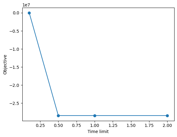
import matplotlib.pyplot as plt

x = runs_table["parameter", "timelimit"]
y = runs_table["solution_scip", "objective"]
plt.plot(x, y, "o-")
plt.xlabel("Time limit")
plt.ylabel("Objective")
plt.show()
Save and Load Experimental Data#
You can save the experiment data at any time using the Experiment.save method.
You can also load saved data using the Experiment.load_from_dir method.
# By default, data is saved under .minto_experiments/ directory
experiment.save()
[2025-08-01 21:48:09] 🎯 Experiment 'scip_exp' completed: 4 runs, total time: 13.1s
exp2 = minto.Experiment.load_from_dir(
    ".minto_experiments/" + experiment.experiment_name
)
[2025-08-01 21:48:10] 🚀 Starting experiment 'scip_exp'
[2025-08-01 21:48:10]   ├─ 📊 Environment: OS: Linux 6.6.93+, CPU: Intel(R) Xeon(R) CPU @ 2.80GHz (4 cores), Memory: 15.6 GB, Python: 3.11.10
[2025-08-01 21:48:10]   ├─ 📊 Environment Information
[2025-08-01 21:48:10]       ├─ OS: Linux 6.6.93+
[2025-08-01 21:48:10]       ├─ Platform: Linux-6.6.93+-x86_64-with-glibc2.35
[2025-08-01 21:48:10]       ├─ CPU: Intel(R) Xeon(R) CPU @ 2.80GHz (4 cores)
[2025-08-01 21:48:10]       ├─ Memory: 15.6 GB
[2025-08-01 21:48:10]       ├─ Architecture: x86_64
[2025-08-01 21:48:10]       ├─ Python: 3.11.10
[2025-08-01 21:48:10]       ├─ Key Package Versions:
exp2.get_run_table()
| solution_scip | parameter | metadata | |||||||
|---|---|---|---|---|---|---|---|---|---|
| objective | feasible | optimality | relaxation | start | name | timelimit | run_id | elapsed_time | |
| run_id | |||||||||
| 0 | 0.000000e+00 | True | 0 | 0 | None | scip | 0.1 | 0 | 0.118683 |
| 1 | -2.841909e+07 | True | 0 | 0 | None | scip | 0.5 | 1 | 0.413625 |
| 2 | -2.841909e+07 | True | 0 | 0 | None | scip | 1.0 | 2 | 0.556057 |
| 3 | -2.841909e+07 | True | 0 | 0 | None | scip | 2.0 | 3 | 1.016498 |
Saving and Load to/from OMMX Archive#
You can save and load data to/from OMMX Archive using the Experiment.save_to_ommx_archive and Experiment.load_from_ommx_archive methods.
artifact = experiment.save_as_ommx_archive("scip_experiment.ommx")
exp3 = minto.Experiment.load_from_ommx_archive("scip_experiment.ommx")
exp3.get_run_table()
[2025-08-01 21:48:26] 🚀 Starting experiment 'scip_exp'
[2025-08-01 21:48:26]   ├─ 📊 Environment: OS: Linux 6.6.93+, CPU: Intel(R) Xeon(R) CPU @ 2.80GHz (4 cores), Memory: 15.6 GB, Python: 3.11.10
[2025-08-01 21:48:26]   ├─ 📊 Environment Information
[2025-08-01 21:48:26]       ├─ OS: Linux 6.6.93+
[2025-08-01 21:48:26]       ├─ Platform: Linux-6.6.93+-x86_64-with-glibc2.35
[2025-08-01 21:48:26]       ├─ CPU: Intel(R) Xeon(R) CPU @ 2.80GHz (4 cores)
[2025-08-01 21:48:26]       ├─ Memory: 15.6 GB
[2025-08-01 21:48:26]       ├─ Architecture: x86_64
[2025-08-01 21:48:26]       ├─ Python: 3.11.10
[2025-08-01 21:48:26]       ├─ Key Package Versions:
| solution_scip | parameter | metadata | |||||||
|---|---|---|---|---|---|---|---|---|---|
| objective | feasible | optimality | relaxation | start | name | timelimit | run_id | elapsed_time | |
| run_id | |||||||||
| 0 | 0.000000e+00 | True | 0 | 0 | None | scip | 0.1 | 0 | 0.118683 |
| 1 | -2.841909e+07 | True | 0 | 0 | None | scip | 0.5 | 1 | 0.413625 |
| 2 | -2.841909e+07 | True | 0 | 0 | None | scip | 1.0 | 2 | 0.556057 |
| 3 | -2.841909e+07 | True | 0 | 0 | None | scip | 2.0 | 3 | 1.016498 |
Summary#
In this tutorial, we learned how to use minto for managing numerical experiments:
Installation is straightforward via pip:
pip install minto
Recording Experimental Data
Used SCIP solver through OMMX interface
Conducted experiments with different time limits (0.1s to 2.0s)
Recorded instance data and solution results systematically
Data Management
Automatic saving with
auto_saving=TrueManual saving with
experiment.save()Data visualization using pandas DataFrame and matplotlib
Results showed objective values converging to -2.92e+07
Data Persistence
Local storage in
.minto_experiments/directoryOMMX archive format support.
Easy data recovery with
load_from_dirandload_from_ommx_archive
This workflow demonstrates minto’s capabilities for structured experimental management in optimization tasks.