Blackbox Optimization

🌐 日本語 | English

Overview

This tutorial shows how to run black-box optimization with JijZept Tools. Black-box optimization is a technique for optimizing a function without detailed knowledge of it. It is used in many fields and has been applied to problems such as materials discovery and hyperparameter optimization. This tutorial introduces two black-box optimization methods:

• FMO (Factorization Machine Optimization)

• BOCS (Bayesian Optimization for Combinatorial Structures)

Let’s get ready to try black-box optimization.

Preparing a black-box function

First, we prepare a black-box function. As a simple example, we consider a QUBO of the form $\( \min_x x Q x^T,~x \in \{0, 1\}^n \)$

import numpy as np


class QuadraticBlackboxFunc:
    def __init__(self, n: int, random_seed: int = 0):
        self.random_state = np.random.RandomState(random_seed)
        Q = self.random_state.uniform(-0.5, 1, (n, n))
        self.Q = (Q + Q.T) / 2
        self.Q[np.abs(self.Q) < 0.08] = 0.0

        noise_variance = 0.1
        num_vars = n
        self.noise_variance = noise_variance
        self.rng = np.random.default_rng(random_seed)
        self.Q = self.rng.normal(0, 1, size=(num_vars, num_vars))

    def __call__(self, x: np.ndarray) -> float:
        return x @ self.Q @ x

Preparing initial data

Let’s prepare initial data for the black-box optimization. Initial data is not strictly required, but providing it can speed up convergence.

Here we generate the initial data randomly.

n = 30
num_init = 10

quad_bf = QuadraticBlackboxFunc(n)

X_init = np.random.choice([0, 1], (num_init, n))
y_init = np.array([quad_bf(x) for x in X_init])

Preparing an optimization solver

Both FMO and BOCS, introduced in this tutorial, build a QUBO matrix as a surrogate function (an approximate model used in place of the true function) and optimize by solving that QUBO matrix, so we need a QUBO solver. Here we prepare one using OpenJij.

Also, since this tutorial uses a QUBO as the black-box function, that QUBO can be solved directly. To compare the performance of the black-box optimization methods, we solve it directly beforehand and store the result in estimated_ground.

import openjij as oj


def solver(Q):
    _Q, _ = Q
    sampler = oj.SASampler()
    response = sampler.sample_qubo(_Q, num_reads=100)
    return response.lowest().states[0]


estimated_ground = quad_bf(solver((quad_bf.Q, None)))

Factorization Machine Optimization

This section shows how to use the black-box optimization method called Factorization Machine Optimization (FMO) with JijZept Tools.

FMO was proposed by [Kitai et al., 2020] and has been applied to a variety of problems such as materials discovery and hyperparameter optimization, demonstrating its effectiveness. Because the original proposal performed the optimization with quantum annealing or simulated annealing, the method is often called FMQA (FM Quantum Annealing) or FMA (FM Annealing). In JijZept Tools a different algorithm can be plugged into the optimization step, so we call it FMO here.

FMO builds a surrogate of the black-box function using a machine-learning model called a Factorization Machine (FM), converts the FM surrogate into QUBO form, and optimizes it. Compared with approaches based on Gaussian processes and the like, FMO is known to be useful for high-dimensional and discrete variables.

Let’s run FMO right away. First, import FMOWorkflow.

from jijzepttools.blackbox_optimization import FMOWorkflow

FMOWorkflow is implemented on top of the JijZept Tools workflow graph, so you can visualize the workflow in a Jupyter Notebook with .workflow.display_workflow().

The n_iter argument of the .run() method specifies the number of optimization iterations. The larger n_iter is, the more iterations run, which improves the optimization accuracy but increases the computation time.

The latent_dim argument of the constructor specifies the dimension of the FM. The larger latent_dim is, the more expressive the FM becomes, at the cost of a higher risk of overfitting.

The flip_postprocess4uniq flag in the constructor specifies whether to post-process the optimization results. Setting this flag to True enables the post-processing, which removes duplicates from the optimization results; without it, the results may contain duplicates. FMO tends to get stuck in local optima, and the post-processing helps it escape a local optimum, continue learning, and optimize more globally. When the flip_postprocess4uniq flag is set, you can see that a step called flip_post_process appears after solve in the workflow. Try toggling flip_postprocess4uniq and confirm that the workflow changes.

fmo_wf = FMOWorkflow(n, latent_dim=5, flip_postprocess4uniq=True)
fmo_wf.workflow.display_workflow("LR")

graph LR;
    _START_["_START_"]
    _START_ --> train
    _END_["_END_"]
    train["train"]
    train --> generate_qubo
    generate_qubo["generate_qubo"]
    generate_qubo --> solve
    solve["solve"]
    solve --> flip_post_process
    flip_post_process["flip_post_process"]
    flip_post_process --> run_blackbox
    run_blackbox["run_blackbox"]
    run_blackbox --> check_iter
    check_iter["check_iter"]
    check_iter -->|"True"| train
    check_iter -->|"False"| _END_

Running FMO

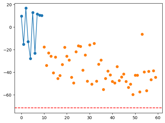
Now let’s run FMO. Calling the .run() method executes the optimization. The third argument is the black-box function; the optimizer calls the black-box function internally as the optimization proceeds.

fmo_results = fmo_wf.run(
    X_init,
    y_init,
    quad_bf,
    solver,
    n_iter=50,
    n_epochs=100,
)

import matplotlib.pyplot as plt

plt.plot(fmo_results[1][:num_init], "-o")
plt.plot(np.arange(num_init, len(fmo_results[1])), fmo_results[1][num_init:], "o")
plt.axhline(estimated_ground, color="red", linestyle="--")

<matplotlib.lines.Line2D at 0x7f56f48df580>

Bayesian Optimization for Combinatorial Structures

This section shows how to use the black-box optimization method called Bayesian Optimization for Combinatorial Structures (BOCS) with JijZept Tools.

BOCS was proposed by [Baptista and Poloczek, 2018] and is known to be effective for combinatorial optimization problems. BOCS obtains a surrogate of the black-box function via Bayesian sparse linear regression. To make the linear regression sparse, it uses a horseshoe prior. JijZept Tools estimates the posterior distribution with Gibbs sampling.

With JijZept Tools you can use BOCS without worrying about the tricky implementation details. Let’s run BOCS in the same way as FMO.

As with FMO, import BOCSWorkflow. BOCSWorkflow also supports the post-processing option, but BOCS is less prone to local optima than FMO, so turning it on is not necessary.

Everything else can be used just like FMO.

from jijzepttools.blackbox_optimization import BOCSWorkflow

bocs_wf = BOCSWorkflow()
bocs_wf.workflow.display_workflow("LR")

graph LR;
    _START_["_START_"]
    _START_ --> train
    _END_["_END_"]
    train["train"]
    train --> generate_qubo
    generate_qubo["generate_qubo"]
    generate_qubo --> solve
    solve["solve"]
    solve --> run_blackbox
    run_blackbox["run_blackbox"]
    run_blackbox --> check_iter
    check_iter["check_iter"]
    check_iter -->|"True"| train
    check_iter -->|"False"| _END_

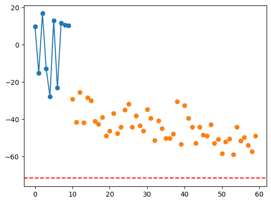
bocs_results = bocs_wf.run(X_init, y_init, quad_bf, solver, n_iter=50, tune=1, draws=1)

import matplotlib.pyplot as plt

plt.plot(bocs_results[1][:num_init], "-o")
plt.plot(np.arange(num_init, len(bocs_results[1])), bocs_results[1][num_init:], "o")
plt.axhline(estimated_ground, color="red", linestyle="--")

<matplotlib.lines.Line2D at 0x7f568311a500>