Qamomile Quickstart Guide

This guide will help you get started with Qamomile quickly, covering installation and basic usage.

Installation

Prerequisites

Before installing Qamomile, ensure you have the following:

• Python 3.10 or higher

• pip (Python package installer)

Installing Qamomile

Install Qamomile using pip:

pip install qamomile

Optional Dependencies

Depending on your needs, you might want to install additional packages:

• For Qiskit integration: pip install "qamomile[qiskit]"

• For Quri Parts integration: pip install "qamomile[quri-parts]"

• For Qutip integration: pip install "qamomile[qutip]"

• For PennyLane integration: pip install "qamomile[pennylane]"

Basic Usages

Let’s walk through a simple example to demonstrate how to use Qamomile.

1. Import Qamomile and JijModeling

import qamomile.core as qm
import jijmodeling as jm
import jijmodeling_transpiler.core as jmt

2. Create a Mathematical Model with JijModeling

# Simple QUBO

Q = jm.Placeholder("Q", ndim=2)
n = Q.len_at(0, latex="n")
x = jm.BinaryVar("x", shape=(n,))

problem = jm.Problem("qubo")
i, j = jm.Element("i", n), jm.Element("j", n)
problem += jm.sum([i, j], Q[i, j] * x[i] * x[j])

problem

\[\begin{split}\begin{array}{cccc}\text{Problem:} & \text{qubo} & & \\& & \min \quad \displaystyle \sum_{i = 0}^{n - 1} \sum_{j = 0}^{n - 1} Q_{i, j} \cdot x_{i} \cdot x_{j} & \\\text{{where}} & & & \\& x & 1\text{-dim binary variable}\\\end{array}\end{split}\]

# Prepare data
instance_data = {
    "Q": [[0.1, 0.2, -0.1],
          [0.2, 0.3, 0.4],
          [-0.1, 0.4, 0.0]]
}

# Compile the problem:
# Substitute the data into the problem.
compiled_instance = jmt.compile_model(problem, instance_data)

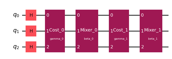
3. Create a Quantum Circuit and a Hamiltonian with Qamomile

qaoa_converter = qm.qaoa.QAOAConverter(compiled_instance)

# Encode to Ising Hamiltonian
qaoa_converter.ising_encode()

# Get the QAOA circuit
qaoa_circuit = qaoa_converter.get_qaoa_ansatz(p=2)
# Get the cost Hamiltonian
qaoa_hamiltonian = qaoa_converter.get_cost_hamiltonian()

4. Transpile to a Quantum Computing SDK (Qiskit or Quri Parts)

In this example, we will use Qiskit.

import qamomile.qiskit as qm_qk

qk_transpiler = qm_qk.QiskitTranspiler()

# Transpile the QAOA circuit to Qiskit
qk_circuit = qk_transpiler.transpile_circuit(qaoa_circuit)
qk_circuit.draw(output="mpl")

# Transpile the QAOA Hamiltonian to Qiskit
qk_hamiltonian = qk_transpiler.transpile_hamiltonian(qaoa_hamiltonian)
qk_hamiltonian

SparsePauliOp(['IIZ', 'IZI', 'ZII', 'IZZ', 'ZIZ', 'ZZI'],
              coeffs=[-0.1 +0.j, -0.45+0.j, -0.15+0.j,  0.1 +0.j, -0.05+0.j,  0.2 +0.j])

5. Run the Quantum Circuit

Run the quantum circuit on a quantum simulator or a real quantum computer.
In this example, we will use the Qiskit.

In Qamomile, the execution of quantum circuits is delegated to the respective SDKs, allowing users to implement this part themselves if they choose to do so. Given that the primary applications of current quantum computers are research and education, we believe that the majority of cases where quantum optimization algorithms are executed will fall under these categories. To avoid turning Qamomile into a black box, the execution of quantum circuits is left to the users, making it easier to customize algorithms.

import qiskit.primitives as qk_pr
import numpy as np
from scipy.optimize import minimize

cost_history = []
def cost_estimator(param_values):
    estimator = qk_pr.StatevectorEstimator()
    job = estimator.run([(qk_circuit, qk_hamiltonian, param_values)])
    result = job.result()[0]
    cost = result.data['evs']
    cost_history.append(cost)
    return cost

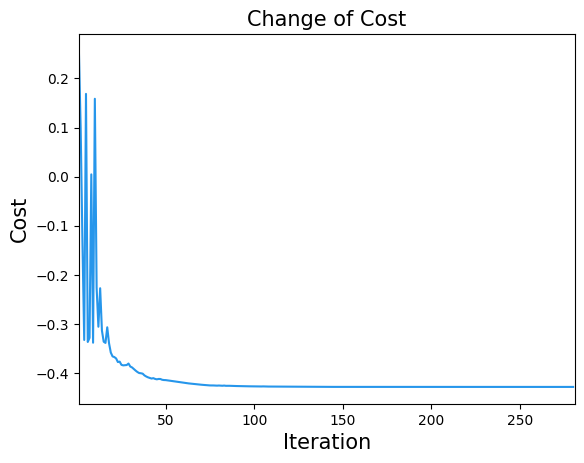
# Run QAOA optimization
result = minimize(
    cost_estimator,
    [np.pi / 4, np.pi / 2, np.pi / 2, np.pi / 4],
    method="COBYLA",
    options={"maxiter": 1000},
)
print(result)

 message: Optimization terminated successfully.
 success: True
  status: 1
     fun: -0.428242617622815
       x: [ 8.005e-01  1.940e+00  1.020e+00  1.509e+00]
    nfev: 281
   maxcv: 0.0

import matplotlib.pyplot as plt

plt.title("Change of Cost", fontsize=15)
plt.xlabel("Iteration", fontsize=15)
plt.ylabel("Cost", fontsize=15)
plt.xlim(1, result.nfev)
plt.plot(cost_history, label="Cost", color="#2696EB")
plt.show()

# Run Optimized QAOA circuit
sampler = qk_pr.StatevectorSampler()
qk_circuit.measure_all()
job = sampler.run([(qk_circuit, result.x)], shots=1000)
job_result = job.result()[0]
qaoa_counts = job_result.data["meas"]
qaoa_counts.get_counts()

{'000': 622, '100': 107, '010': 8, '001': 226, '101': 35, '011': 1, '111': 1}

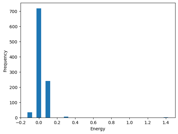
6. Decode the Result

After running the quantum circuit, decode the result to obtain the solution.

from collections import defaultdict
import matplotlib.pyplot as plt

sampleset = qaoa_converter.decode(qk_transpiler, job_result.data["meas"])

# Initialize a dictionary to accumulate occurrences for each energy value
frequencies = defaultdict(int)

# Define the precision to which you want to round the energy values
for sample in sampleset:
    energy = round(sample.eval.objective, ndigits = 3)  
    frequencies[energy] += sample.num_occurrences

plt.bar(frequencies.keys(), frequencies.values(), width=0.05)
plt.xlabel('Objective')
plt.ylabel('Frequency')
plt.show()