QAOA for the Vertex Cover#
In this section, we will solve the Vertex Cover Problem using QAOA with the help of the JijModeling and Qamomile libraries.
First, let’s install and import the main libraries we will be using.
# !pip install qamomile[qiskit,quri-parts]
# !pip install pylatexenc
import qamomile.core as qm
import jijmodeling as jm
import jijmodeling_transpiler.core as jmt
import networkx as nx
import matplotlib.pyplot as plt
The Vertex Cover Problem#
First, let’s review the definition of the Vertex Cover Problem. In an undirected graph \(G = (V, E)\), a vertex set \(S \subseteq V\) is called a vertex cover if for every edge \(e = (i, j) \in E\), either \(i \in S\) or \(j \in S\) holds. The Vertex Cover Problem is the problem of finding a vertex cover \(S\) with the smallest possible number of elements.
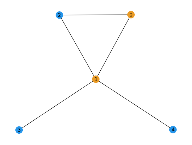
As an example, consider the minimum vertex cover of the following graph. Let \(S = \{0, 1\}\). In this case, every edge of the graph has at least one in either vertex \(0\) or vertex \(1\), so \(S\) is a vertex cover set. Furthermore, in the graph we are considering, there is no vertex cover \(S\) with only one element, so \(\{0, 1\}\) is indeed the minimum vertex cover.
G = nx.Graph()
G.add_nodes_from([0, 1, 2, 3, 4])
G.add_edges_from([(0, 1), (0, 2), (1, 2), (1, 3), (1, 4)])
positions = nx.spring_layout(G)
color = ["#2696EB"] * 5
color[0] = color[1] = "#EA9b26"
nx.draw(G, node_color=color, pos=positions, with_labels=True)
Formulation of the Vertex Cover Problem#
Let’s consider the formulation of the Vertex Cover Problem.
We define a binary variable \(x_i\) such that \(x_i = 1\) if vertex \(i\) is included in \(S\), and \(x_i = 0\) otherwise. The objective function, which represents the size of \(S\), can be expressed as follows.
The constraint is that all edges must be covered, meaning that for each edge, at least one of its endpoints must be included in \(S\). This can be formulated as:
In summary, the Vertex Cover Problem can be formulated as follows:
Creating Problem Model using JijModeling#
We describe the above formulation and then using JijModeling to create the problem model. Placeholder defines the values to be substituted as data, BinaryVar defines the decision variables, and Element defines the indices used in the summation. By checking the output, we can confirm that the formulation is correct.
def vertex_cover_problem() -> jm.Problem:
    # define variables
    V = jm.Placeholder("V")
    E = jm.Placeholder("E", ndim=2)
    x = jm.BinaryVar("x", shape=(V,))
    i = jm.Element("i", belong_to=(0, V))
    e = jm.Element("e", belong_to=E)

    # set problem
    problem = jm.Problem("Vertex Cover Problem")
    # ensure that at least one vertex of each edge is included in the cover
    problem += jm.Constraint("cover", x[e[0]] + x[e[1]] >= 1, forall=e)
    # minimize the number of vertices included in the cover
    problem += jm.sum(i, x[i])

    return problem


problem = vertex_cover_problem()
problem
Preparing Instance Data#
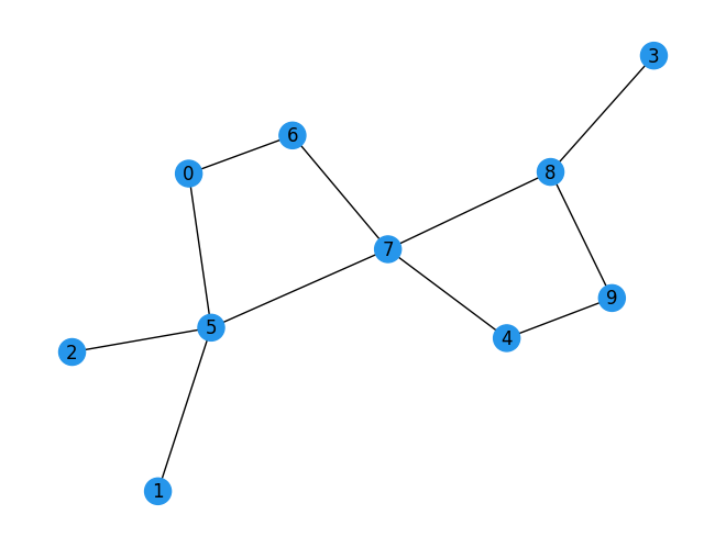
Next, we will solve the Vertex Cover Problem for the following graph. The data for the specific problem being solved is referred to as instance data.
G = nx.Graph()
G.add_nodes_from([0, 1, 2, 3, 4, 5, 6, 7, 8, 9])
G.add_edges_from(
    [
        (0, 6),
        (0, 5),
        (1, 5),
        (2, 5),
        (3, 8),
        (4, 9),
        (4, 7),
        (5, 7),
        (6, 7),
        (7, 8),
        (8, 9),
    ]
)
positions = nx.spring_layout(G)
color = ["#2696EB"] * G.number_of_nodes()
nx.draw(G, node_color=color, pos=positions, with_labels=True)
Creating a Compiled Instance#
We perform compilation using the JijModeling-Transpiler by providing the formulation and the instance data prepared earlier. This process yields an intermediate representation of the problem with the instance data substituted.
inst_E = [list(edge) for edge in G.edges]
num_nodes = G.number_of_nodes()
instance_data = {"V": num_nodes, "E": inst_E}
num_qubits = num_nodes
compiled_instance = jmt.compile_model(problem, instance_data)
Converting Compiled Instance to QAOA Circuit and Hamiltonian#
We generate the QAOA circuit and Hamiltonian from the compiled Instance. The converter used to generate these is qm.qaoa.QAOAConverter.
By creating an instance of this class and using ising_encode, you can internally generate the Ising Hamiltonian from the compiled Instance. Parameters that arise during the conversion to QUBO can also be set here. If not set, default values are used.
Once the Ising Hamiltonian is generated, you can generate the QAOA quantum circuit and the Hamiltonian respectively. These can be executed using the get_qaoa_ansatz and get_cost_hamiltonian methods. The number of QAOA layers, \(p\), is fixed to be \(4\) here.
qaoa_converter = qm.qaoa.QAOAConverter(compiled_instance)
# Encode to Ising Hamiltonian
qaoa_converter.ising_encode()
# Get the QAOA circuit
qaoa_circuit = qaoa_converter.get_qaoa_ansatz(p=3)
# Get the cost Hamiltonian
qaoa_hamiltonian = qaoa_converter.get_cost_hamiltonian()
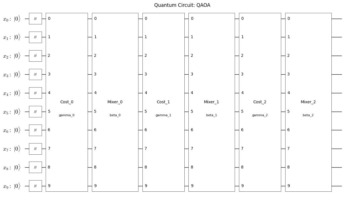
Visualization of QAOA Circuit#
Qamomile provides a method to visualize the quantum circuit. You can use the plot_quantum_circuit function to visualize the QAOA quantum circuit.
from qamomile.core.circuit.drawer import plot_quantum_circuit

plot_quantum_circuit(qaoa_circuit)
Converting the Obtained QAOA Circuit and Hamiltonian for Qiskit#
Here, we generate the Qiskit’s QAOA circuit and Hamiltonian using the qamomile.qiskit.QiskitTranspiler converters. By utilizing the two methods,QiskitTranspiler.transpile_circuit and QiskitTranspiler.transpile_hamiltonian, we can transform the QAOA circuit and Hamiltonian into a format compatible with Qiskit. This allows us to leverage Qiskit’s quantum computing framework to execute and analyze.
import qamomile.qiskit as qm_qk

qk_transpiler = qm_qk.QiskitTranspiler()
# Transpile the QAOA circuit to Qiskit
qk_circuit = qk_transpiler.transpile_circuit(qaoa_circuit)
# Transpile the QAOA Hamiltonian to Qiskit
qk_hamiltonian = qk_transpiler.transpile_hamiltonian(qaoa_hamiltonian)
qk_hamiltonian
SparsePauliOp(['IIIIIIIIIZ', 'IIIIIZIIII', 'IIIIZIIIII', 'IIIZIIIIII', 'IIZIIIIIII', 'IZIIIIIIII', 'ZIIIIIIIII', 'IIIZIIIIIZ', 'IIIIZIIIIZ', 'IIIIZIIIZI', 'IIIIZIIZII', 'IZIIIIZIII', 'ZIIIIZIIII', 'IIZIIZIIII', 'IIZIZIIIII', 'IIZZIIIIII', 'IZZIIIIIII', 'ZZIIIIIIII'],
              coeffs=[0.5+0.j, 0.5+0.j, 1.5+0.j, 0.5+0.j, 1.5+0.j, 1. +0.j, 0.5+0.j, 0.5+0.j,
 0.5+0.j, 0.5+0.j, 0.5+0.j, 0.5+0.j, 0.5+0.j, 0.5+0.j, 0.5+0.j, 0.5+0.j,
 0.5+0.j, 0.5+0.j])
Running QAOA#
We run QAOA to optimize the parameters. Here, we use COBYLA as the optimizer.
import qiskit.primitives as qk_pr
import numpy as np
from scipy.optimize import minimize

cost_history = []
estimator = qk_pr.StatevectorEstimator()


# Cost estimator function
def estimate_cost(param_values):
    try:
        job = estimator.run([(qk_circuit, qk_hamiltonian, param_values)])
        result = job.result()[0]
        cost = result.data["evs"]
        cost_history.append(cost)
        return cost
    except Exception as e:
        print(f"Error during cost estimation: {e}")
        return np.inf


# Initial parameters for QAOA
initial_params = [
    np.pi / 8,
    np.pi / 4,
    3 * np.pi / 8,
    np.pi / 2,
    np.pi / 2,
    3 * np.pi / 8,
]

# Run QAOA optimization with COBYLA
result = minimize(
    estimate_cost,
    initial_params,
    method="COBYLA",
    options={"maxiter": 1500},
)

print(result)
 message: Optimization terminated successfully.
 success: True
  status: 1
     fun: -3.8319489423814184
       x: [ 7.111e-01  8.882e-02  1.106e+00  2.621e+00  2.031e+00
            1.371e+00]
    nfev: 321
   maxcv: 0.0
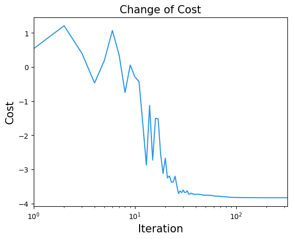
Result Visualization#
By repeating the optimization, we can observe that the energy decreases and converges.
plt.title("Change of Cost", fontsize=15)
plt.xlabel("Iteration", fontsize=15)
plt.ylabel("Cost", fontsize=15)
plt.xscale("log")
plt.xlim(1, result.nfev)
plt.plot(cost_history, label="Cost", color="#2696EB")
plt.show()
Now, let’s run the Optimized paremeter on qiskit StatevectorSampler.
# Run Optimized QAOA circuit
sampler = qk_pr.StatevectorSampler()
qk_circuit.measure_all()
job = sampler.run([(qk_circuit, result.x)], shots=1000)
job_result = job.result()[0]
qaoa_counts = job_result.data["meas"]
Evaluating the Results#
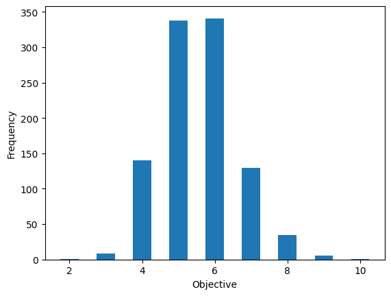
From the job counts obtained earlier, we can transfer them to a sampleset by qaoa_converter.decode.
The sampleset can select only the feasible solutions and then we examine the distribution of the objective function values.
from collections import defaultdict
import matplotlib.pyplot as plt

sampleset = qaoa_converter.decode(qk_transpiler, job_result.data["meas"])

# Initialize a dictionary to accumulate occurrences for each energy value
frequencies = defaultdict(int)

# Define the precision to which you want to round the energy values
for sample in sampleset:
    energy = round(sample.eval.objective, ndigits = 3)
    frequencies[energy] += sample.num_occurrences

plt.bar(frequencies.keys(), frequencies.values(), width=0.5)
plt.xlabel('Objective')
plt.ylabel('Frequency')
plt.show()
Plotting the Solution#
From the obtained results, we select one solution that minimizes the objective function value and plot it. (The orange vertices are the vertices included in the vertex cover.)
def plot_graph_coloring(graph: nx.Graph, sampleset: jm.SampleSet):
    # extract feasible solution
    lowests = sampleset.lowest()
    if len(lowests) == 0:
        print("No feasible solution found ...")
    else:
        best_sol = lowests[0]

        # initialize vertex color list
        node_colors = ["#2696EB"] * instance_data["V"]
        # set vertex color
        for t in best_sol.var_values["x"].values.keys():
            node_colors[t[0]] = "#EA9b26"
        # make figure
        nx.draw_networkx(graph, node_color=node_colors, pos=positions, with_labels=True)
        plt.show()


plot_graph_coloring(G, sampleset)
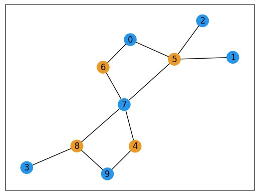
Indeed, we can see that a vertex cover has been obtained.