Fermionic QAOA for Portfolio Optimization#
In this tutorial, we will solve the portfolio optimization using the Femionic Quantum Approximate Optimization Algorithm (FQAOA).
import copy
from itertools import combinations
import numpy as np
import matplotlib.pyplot as plt
import scipy.optimize as opt
import networkx as nx
import qiskit.primitives as qk_pr

import jijmodeling as jm
import ommx.v1
from ommx_pyscipopt_adapter import OMMXPySCIPOptAdapter

import qamomile.core as qm
from qamomile.core.circuit.circuit import ParametricTwoQubitGate
from qamomile.qiskit import QiskitTranspiler
from qamomile.core.circuit.drawer import plot_quantum_circuit
from qamomile.core.converters.fqaoa import FQAOAConverter
from qamomile.core.ising_qubo import IsingModel

rng = np.random.default_rng()
Portfolio optimization#
The portfolio optimization problem is the problem of finding the optimal portfolio in asset investment. Here, we use a formulation based on the most well-known Markowitz model. The Markowitz model aims to maximize returns while minimizing risk. Risk is given by the variance \(\mu_{ij}\) between assets, and return is represented by \(h_i\). The combination of these two forms the cost function:
Here, \(\lambda : (0 < \lambda < 1)\) is a parameter that adjusts the balance between return and risk. The solution to the portfolio optimization is obtained by solving the minimization problem of this function. The decision variable \(w_i\) represents the position for the \(i\)-th asset. When \(w_i = 0\), the stock is not held (no position), and when \(w_i = \pm 1\), the stock is held in a long or short position. Furthermore, if there is a limit on the number of assets that can be held, it can be expressed with the following constraint conditions:
Here, \(D\) is the total number of assets that can be held. In this case, the portfolio optimization problem becomes a constrained combinatorial optimization problem.
Constructing the Mathematical Model#
The mathematical model of portfolio optimization is implemented using JijModeling. Since QAOA is an algorithm for QUBO, the integer variables \(w = \{-1, 0 , 1\}^N\) need to be converted into binary variables \(x = \{0,1\}\). Here, two binary variables are used for each variable \(w_i\), and \(w_i = 1 - x_{i,1} - x_{i,2}\) is used to represent it.
First, we will implement the mathematical model of the portofolio optimization problem using JijModeling.
def create_potofolio_optimzation_problem():
    N = jm.Placeholder("N") # The number of decision variables
    D = jm.Placeholder("D") # The number of bits that need to encode an integer variable into binary variables
    M = jm.Placeholder("M")
    lam = jm.Placeholder("lam") # A parameter that adjusts the balance between risk and return
    lam.set_latex("\lambda")
    sigma = jm.Placeholder("sigma", ndim=2) # A covariance matrix that represents the normalized asset returns
    sigma.set_latex("\sigma")
    mu = jm.Placeholder("mu", ndim=1) # A returns vector that represents the normalized average asset
    mu.set_latex("\mu")

    x = jm.BinaryVar("x", shape=(N,D))
    l = jm.Element("l", belong_to=(0,N))
    l_dash = jm.Element("l'", belong_to=(0,N))
    d = jm.Element("d", belong_to=(0,D))
    d_dash = jm.Element("d'", belong_to=(0,D))

    problem = jm.Problem("Portfolio Optimization", sense=jm.ProblemSense.MINIMIZE)

    problem += -lam * jm.sum([l, l_dash], sigma[l,l_dash] * jm.sum([d, d_dash], (x[l,d]-0.5) * (x[l_dash, d_dash]-0.5))) + (1-lam) * jm.sum(l, mu[l] * jm.sum(d, (x[l,d]-0.5)))

    problem += jm.Constraint("the total number of stock holdings", jm.sum([l,d], x[l,d])==N-M)

    return problem

problem_minimize = create_potofolio_optimzation_problem()
problem_minimize
We will now prepare the problem to be solved and perform compilation using JijModeling.Interpreter and ommx.v1.Instance.
num_integer = 5
num_bit = 2
num_stock = 3
sigma = rng.uniform(-0.1, 0.1, size=(num_integer, num_integer))
mu = rng.uniform(-1.0, 1.0, size=num_integer)
lam = 0.1

instance_data = {"N": num_integer, "D": num_bit, "M": num_stock, "lam": lam, "sigma": sigma, "mu": mu}
interpreter = jm.Interpreter(instance_data)
instance: ommx.v1.Instance = interpreter.eval_problem(problem_minimize)
Implementing FQAOA using Qamomile#
We generate the FQAOA circuit and Hamiltonian from the compiled Instance. The converter used to generate these is qm.fqaoa.FQAOAConverter.
num_fermions = num_integer - num_stock # N - M
p = 10
fqaoa_converter = FQAOAConverter(instance, num_fermions=num_fermions, normalize_model=False)
fqaoa_circuit = fqaoa_converter.get_fqaoa_ansatz(p)
fqaoa_cost = fqaoa_converter.get_cost_hamiltonian()
Run FQAOA using Qiskit#
Here, we generate the Qiskit’s QAOA circuit and Hamiltonian using the qamomile.qiskit.QiskitTranspiler converters. By utilizing the two methods,QiskitTranspiler.transpile_circuit and QiskitTranspiler.transpile_hamiltonian, we can transform the QAOA circuit and Hamiltonian into a format compatible with Qiskit.
qk_transpiler = QiskitTranspiler()
qk_circuit = qk_transpiler.transpile_circuit(fqaoa_circuit)
qk_cost = qk_transpiler.transpile_hamiltonian(fqaoa_cost)
We run FQAOA to optimize the parameters. Here, we use the BFGS method as the optimizer.
init_params = [rng.uniform(0.0, 2.0*np.pi) for i in range(2*p)]
estimator = qk_pr.StatevectorEstimator()

cost_history = []
def estinamate_cost(params):
    job = estimator.run([(qk_circuit, qk_cost, params)])
    job_result = job.result()
    cost = job_result[0].data['evs']
    cost_history.append(cost)
    return cost

result = opt.minimize(estinamate_cost, init_params, method="BFGS")
result
  message: Optimization terminated successfully.
  success: True
   status: 0
      fun: -0.7737245241429906
        x: [ 1.148e-01  1.706e+00 ... -3.230e+00  3.157e+00]
      nit: 223
      jac: [ 5.394e-06  4.470e-06 ... -2.608e-07 -1.788e-07]
 hess_inv: [[ 2.887e+00 -4.986e-01 ... -7.918e+00  5.656e+00]
            [-4.986e-01  6.725e-01 ...  2.286e+00 -1.704e+00]
            ...
            [-7.918e+00  2.286e+00 ...  1.706e+02 -3.817e+01]
            [ 5.656e+00 -1.704e+00 ... -3.817e+01  4.878e+01]]
     nfev: 5040
     njev: 240
Result Visualization#
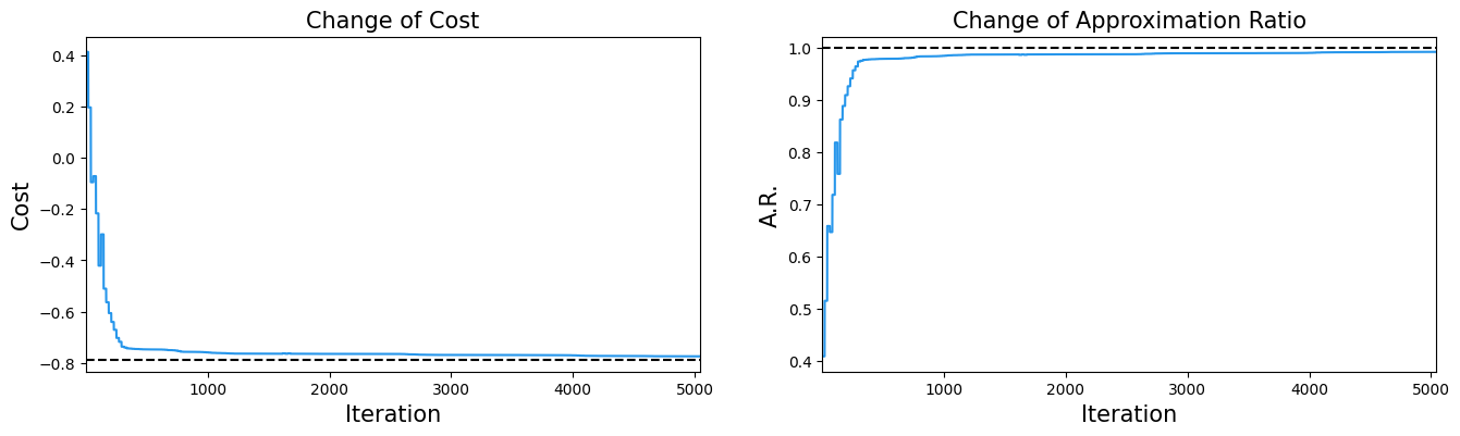
We visualize the optimization process. We plot the changes in the cost function and the approximation ratio. The approximation ratio is an indicator of how close the algorithm’s solution \(\boldsymbol{x}\) is to the optimal solution \(\boldsymbol{x}^*\).
Here, \(C_{\max}\) is the maximum energy value. First, we compute the maximum and minimum energy of the transformed Ising Hamiltonian by brute-force search.
num_qubits = num_integer * num_bit
ising = fqaoa_converter.ising

energy_list = []
state_list = []
for id_list in combinations(np.arange(num_qubits), num_fermions):
    state = [-1 if x in id_list else 1 for x in range(num_qubits)]
    objective_value = ising.calc_energy(state) - ising.constant
    energy_list.append(objective_value)
    state_list.append(state)

energy_list = np.array(energy_list)
min_energy = energy_list.min()
max_energy = energy_list.max()
Using the obtained maximum and minimum energy values, we calculate the approximation ratio.
approx_ratio = 1.0 - np.abs(np.array(cost_history)-min_energy) / np.abs(max_energy - min_energy)

fig1, ax1 = plt.subplots(1, 2, figsize=(16,4))

ax1[0].plot(cost_history, label="Cost", color="#2696EB")
ax1[0].axhline(min_energy, linestyle="--", color="black")
ax1[0].set_xlim(1, result.nfev)
ax1[0].set_xlabel("Iteration", fontsize=15)
ax1[0].set_ylabel("Cost", fontsize=15)
ax1[0].set_title("Change of Cost", fontsize=15)

ax1[1].plot(approx_ratio, label="AR", color="#2696EB")
ax1[1].axhline(1.0, linestyle="--", color="black")
ax1[1].set_xlim(1, result.nfev)
ax1[1].set_xlabel("Iteration", fontsize=15)
ax1[1].set_ylabel("A.R.", fontsize=15)
ax1[1].set_title("Change of Approximation Ratio", fontsize=15)

plt.show()
Evaluating the Results#
From the job counts obtained earlier, we can transfer them to a sampleset by qm.fqaoa.FQAOAConverter.decode.
The sampleset can select only the feasible solutions and then we examine the distribution of the objective function values.
solution = OMMXPySCIPOptAdapter.solve(instance)
min_objective = solution.objective

num_samples = 10000
sampler = qk_pr.StatevectorSampler()
qk_circuit.measure_all()
job = sampler.run([(qk_circuit, result.x)], shots=num_samples)
job_result = job.result()[0]
qaoa_counts = job_result.data["meas"]

sampleset = fqaoa_converter.decode(qk_transpiler, job_result.data["meas"])
plot_data = {}
energies = []
frequencies = []
for sample_id in sampleset.sample_ids:
    sample = sampleset.get(sample_id)
    energies.append(sample.objective)
    frequencies.append(1)

# Group by energy to get frequencies
from collections import defaultdict
energy_freq = defaultdict(int)
for energy in energies:
    energy_freq[energy] += 1

fig2, ax2 = plt.subplots(figsize=(8,4))
ax2.bar(energy_freq.keys(), energy_freq.values(), width=0.05, color='#2696EB')
ax2.axvline(min_objective, linestyle="--", color="red", label='Optimal solution')
ax2.set_title("cost distribution of feasible solution", fontsize=15)
ax2.set_ylabel("Frequency", fontsize=15)
ax2.set_xlabel("Energy", fontsize=15)
ax2.legend()
plt.show()
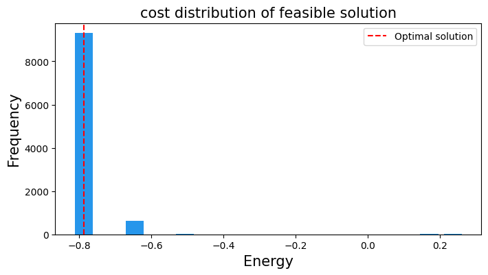
Of course, ommx.v1.SampleSet can be used to verify whether the samples satisfy the constraints of the original problem. The output states of FQAOA all satisfy the constraints.
df_sampleset = sampleset.summary
print(f"feasible solutions: {(df_sampleset['feasible'] == True).sum()}/{num_samples}")
print(f"infeasible solutions: {(df_sampleset['feasible'] == False).sum()}/{num_samples}")
feasible solutions: 10000/10000
infeasible solutions: 0/10000