OpenJij SA Parameter Dependency Experiment with MINTO

This notebook is a simple experiment to see how the parameters of the Simulated Annealing (SA) algorithm in OpenJij affect the performance of the algorithm.

The SA algorithm has temperature as a parameter, and OpenJij automatically sets this temperature based on the coefficients of QUBO or Ising models. Let’s verify how effective these automatic parameter settings are by using grid search.

Even in grid search cases, using MINTO for logging allows us to easily convert the data to pandas.DataFrame for visualization. This helps us analyze the relationship between different parameter combinations and their impact on solution quality and execution time.

import openjij as oj
import numpy as np
import minto
import matplotlib.pyplot as plt
import seaborn as sns

1. Create Random QUBO

def random_qubo(n, sparsity=0.5):
    q = np.random.uniform(-1, 1, (n, n))
    q = (q + q.T) / 2
    zero_num = int(n**2 * sparsity)
    zero_i = np.random.choice(n, zero_num, replace=True)
    zero_j = np.random.choice(n, zero_num, replace=True)
    q[zero_i, zero_j] = 0
    q[zero_j, zero_i] = 0
    qubo = {}
    for i in range(n-1):
        for j in range(i, n):
            qubo[(i, j)] = q[i, j]
            qubo[(j, i)] = q[j, i]
    return qubo

n = 200
q = random_qubo(n)

2. Run with default parameters

In OpenJij, you can check the automatically configured SA parameters through .info['schedule'] in the return value of .sample_qubo. These parameters are stored under the key ‘schedule’ since the temperature settings in SA are referred to as the annealing schedule.

sampler = oj.SASampler()
response = sampler.sample_qubo(q)
schedule = response.info["schedule"]
schedule

{'beta_max': 23419.346516449466,
 'beta_min': 0.16080952839167884,
 'num_sweeps': 1000}

3. Grid search with MINTO

Let’s see how the optimization results change by varying the inverse temperature parameters of SA. We’ll include OpenJij’s default parameters in our search range for comparison.

The important values from OpenJij’s results are stored using .log_parameter method. The complete OpenJij response object is also saved using .log_object method with .to_serializable.

exp = minto.Experiment(auto_saving=False, verbose_logging=False)

# log_object accepts only serializable objects
# so we need to convert qubo to serializable object
qubo_edges = [[i, j] for i, j in q.keys()]
qubo_vales = [q[i, j] for i, j in qubo_edges]
exp.log_global_object("qubo", {"qubo_edges": qubo_edges, "qubo_vales": qubo_vales})

beta_min_list = [schedule["beta_min"], 0.1, 1.0, 2.0, 3.0, 4.0, 5.0]
beta_max_list = [10.0, 20, 30.0, 40.0, 50.0, 12404, schedule["beta_max"]]
num_reads = 300

exp.log_global_parameter("num_reads", num_reads)

for beta_min in beta_min_list:
    for beta_max in beta_max_list:
        run = exp.run()
        with run:
            sampler = oj.SASampler()
            response = exp.log_solver(sampler.sample_qubo)(q, num_reads=num_reads, beta_min=beta_min, beta_max=beta_max)
            beta_min = response.info["schedule"]["beta_min"]
            beta_max = response.info["schedule"]["beta_max"]
            run.log_parameter("beta_min", beta_min)
            run.log_parameter("beta_max", beta_max)
            run.log_object("response", response.to_serializable())
            energies = response.energies
            run.log_parameter("mean_energy", np.mean(energies))
            run.log_parameter("std_energy", np.std(energies))
            run.log_parameter("min_energy", np.min(energies))
            run.log_parameter("exec_time", response.info["execution_time"])

run_table = exp.get_run_table()
run_table

	parameter								metadata
	solver_name	num_reads	beta_min	beta_max	mean_energy	std_energy	min_energy	exec_time	run_id	elapsed_time
run_id
0	sample_qubo	300	0.16081	10.000000	-400.824501	0.484598	-400.996724	7320.595947	0	2.307072
1	sample_qubo	300	0.16081	20.000000	-400.856420	0.430543	-400.996724	5654.832770	1	1.786222
2	sample_qubo	300	0.16081	30.000000	-400.879704	0.426166	-400.996724	5079.307230	2	1.609961
3	sample_qubo	300	0.16081	40.000000	-400.832098	0.587155	-400.996724	5136.469184	3	1.631495
4	sample_qubo	300	0.16081	50.000000	-400.822022	0.554464	-400.996724	4789.121793	4	1.520938
5	sample_qubo	300	0.16081	12404.000000	-400.751895	0.727066	-400.996724	2806.774479	5	0.923433
6	sample_qubo	300	0.16081	23419.346516	-400.866998	0.390925	-400.996724	3326.943347	6	1.121839
7	sample_qubo	300	0.10000	10.000000	-400.846235	0.430128	-400.996724	8428.824636	7	2.629364
8	sample_qubo	300	0.10000	20.000000	-400.871184	0.487043	-400.996724	8039.599841	8	2.506840
9	sample_qubo	300	0.10000	30.000000	-400.902827	0.408157	-400.996724	7164.250151	9	2.246223
10	sample_qubo	300	0.10000	40.000000	-400.846486	0.518750	-400.996724	7217.507659	10	2.281367
11	sample_qubo	300	0.10000	50.000000	-400.871300	0.414777	-400.996724	7409.847616	11	2.359738
12	sample_qubo	300	0.10000	12404.000000	-400.763619	0.681448	-400.996724	3967.293037	12	1.282385
13	sample_qubo	300	0.10000	23419.346516	-400.798245	0.626965	-400.996724	3634.867900	13	1.176097
14	sample_qubo	300	1.00000	10.000000	-400.876989	0.393766	-400.996724	1814.065554	14	0.634887
15	sample_qubo	300	1.00000	20.000000	-400.913995	0.284922	-400.996724	1642.247617	15	0.582999
16	sample_qubo	300	1.00000	30.000000	-400.917115	0.326967	-400.996724	1575.222380	16	0.557419
17	sample_qubo	300	1.00000	40.000000	-400.897331	0.327189	-400.996724	1555.458699	17	0.551024
18	sample_qubo	300	1.00000	50.000000	-400.873310	0.435403	-400.996724	1642.721627	18	0.583553
19	sample_qubo	300	1.00000	12404.000000	-400.782218	0.736565	-400.996724	1296.150597	19	0.478549
20	sample_qubo	300	1.00000	23419.346516	-400.752245	0.750855	-400.996724	1259.816277	20	0.470215
21	sample_qubo	300	2.00000	10.000000	-400.275671	1.410707	-400.996724	1793.180684	21	0.643176
22	sample_qubo	300	2.00000	20.000000	-400.273639	1.434920	-400.996724	1236.816780	22	0.457378
23	sample_qubo	300	2.00000	30.000000	-400.321825	1.388250	-400.996724	1289.589597	23	0.536138
24	sample_qubo	300	2.00000	40.000000	-400.343488	1.390948	-400.996724	1224.864280	24	0.484222
25	sample_qubo	300	2.00000	50.000000	-400.077238	1.566290	-400.996724	1541.285166	25	0.563982
26	sample_qubo	300	2.00000	12404.000000	-399.901651	1.722083	-400.996724	999.701380	26	0.382907
27	sample_qubo	300	2.00000	23419.346516	-399.657682	1.894547	-400.996724	981.944184	27	0.378587
28	sample_qubo	300	3.00000	10.000000	-399.902580	1.671486	-400.996724	1225.427640	28	0.455167
29	sample_qubo	300	3.00000	20.000000	-399.912649	1.695561	-400.996724	1137.585579	29	0.425236
30	sample_qubo	300	3.00000	30.000000	-399.732836	1.784211	-400.996724	1088.030837	30	0.407760
31	sample_qubo	300	3.00000	40.000000	-399.539447	1.908955	-400.996724	1708.495144	31	0.629259
32	sample_qubo	300	3.00000	50.000000	-399.949886	1.626373	-400.996724	1114.417623	32	0.422720
33	sample_qubo	300	3.00000	12404.000000	-399.170922	2.257485	-400.996724	994.269463	33	0.387057
34	sample_qubo	300	3.00000	23419.346516	-399.142392	2.283888	-400.996724	1039.375593	34	0.399291
35	sample_qubo	300	4.00000	10.000000	-399.468546	2.045237	-400.996724	1394.524324	35	0.503925
36	sample_qubo	300	4.00000	20.000000	-399.663096	1.891882	-400.996724	1161.613157	36	0.432853
37	sample_qubo	300	4.00000	30.000000	-399.223775	2.156165	-400.996724	1117.509577	37	0.422596
38	sample_qubo	300	4.00000	40.000000	-399.244652	2.301861	-400.996724	1076.702520	38	0.406730
39	sample_qubo	300	4.00000	50.000000	-399.255288	2.244128	-400.996724	1163.474183	39	0.441943
40	sample_qubo	300	4.00000	12404.000000	-397.954240	2.918028	-400.996724	957.726344	40	0.372531
41	sample_qubo	300	4.00000	23419.346516	-398.225302	2.876724	-400.996724	968.979167	41	0.374739
42	sample_qubo	300	5.00000	10.000000	-399.310750	2.116636	-400.996724	1240.366690	42	0.463734
43	sample_qubo	300	5.00000	20.000000	-398.984841	2.656825	-400.996724	1092.965307	43	0.412869
44	sample_qubo	300	5.00000	30.000000	-398.737762	2.400117	-400.996724	1099.189563	44	0.417825
45	sample_qubo	300	5.00000	40.000000	-398.967248	2.366554	-400.996724	1095.224897	45	0.413972
46	sample_qubo	300	5.00000	50.000000	-398.820041	2.552062	-400.996724	1057.486363	46	0.400985
47	sample_qubo	300	5.00000	12404.000000	-398.017529	3.109239	-400.996724	1554.896517	47	0.613324
48	sample_qubo	300	5.00000	23419.346516	-397.548366	3.214462	-400.996724	1155.085567	48	0.456844

4. Visualizing the results

Convert the run_table to a format suitable for heatmap visualization using pivot method.

MINTO’s .get_run_table() returns a DataFrame with double-header, so we use 'parameter' key to extract the relevant DataFrame and then transform it for heatmap visualization.

param_table = run_table["parameter"].pivot(index="beta_min", columns="beta_max", values="mean_energy")
param_table

beta_max	10.000000	20.000000	30.000000	40.000000	50.000000	12404.000000	23419.346516
beta_min
0.10000	-400.846235	-400.871184	-400.902827	-400.846486	-400.871300	-400.763619	-400.798245
0.16081	-400.824501	-400.856420	-400.879704	-400.832098	-400.822022	-400.751895	-400.866998
1.00000	-400.876989	-400.913995	-400.917115	-400.897331	-400.873310	-400.782218	-400.752245
2.00000	-400.275671	-400.273639	-400.321825	-400.343488	-400.077238	-399.901651	-399.657682
3.00000	-399.902580	-399.912649	-399.732836	-399.539447	-399.949886	-399.170922	-399.142392
4.00000	-399.468546	-399.663096	-399.223775	-399.244652	-399.255288	-397.954240	-398.225302
5.00000	-399.310750	-398.984841	-398.737762	-398.967248	-398.820041	-398.017529	-397.548366

sns.heatmap(param_table, annot=True, fmt="1.1f", cmap="coolwarm")
plt.xlabel("beta_max")
plt.ylabel("beta_min")
plt.title("mean energy")
plt.show()

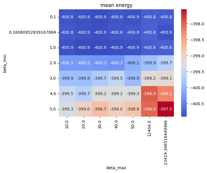
5. Result Analysis

Looking at the results, OpenJij’s default parameters are good enough for this problem.

Let’s examine another perspective. In OpenJij’s algorithm, when a spin flip is rejected, no calculation is performed. When a spin flip occurs, the energy difference is calculated. Therefore, if the temperature is high (inverse temperature beta is low) for a long period, the number of spin flips increases, leading to increased computation time.

As a result, the computation time varies depending on the temperature settings. Let’s visualize these results. OpenJij’s computation time is measured in microseconds.

exec_table = run_table["parameter"].pivot(
    index="beta_min", columns="beta_max", values="exec_time"
)
sns.heatmap(exec_table, annot=True, cmap="coolwarm", annot_kws={"size": 8})
plt.xlabel("beta_max")
plt.ylabel("beta_min")
plt.title("Execution time")
plt.show()

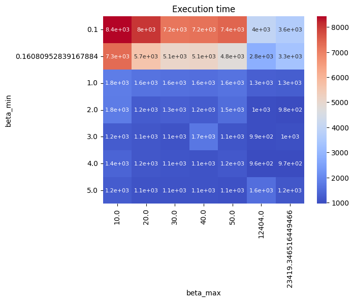
Analysis of OpenJij’s Default Parameters

Unfortunately, from the perspective of computation time, OpenJij’s default parameters do not appear to be optimal. The combination of beta_min=0.3 and beta_max=20~40 seems to be the best. This setting also yields good results in terms of computation time.

We hope that OpenJij’s default parameters will be improved in the future.

As shown here, using minto makes it easy to tune the parameters of heuristic algorithms like OpenJij.

from openjij._version import __version__ as oj_version
print(f"OpenJij version: {oj_version}")

OpenJij version: 0.11.2