QUBO’s hyper parameter search

This notebook is a simple example of how to use MINTO to explore the hyperparameter space of a QUBO model. For this example, we will handle the Traveling Salesman Problem with quadratic assignment formulation. For more details about the Traveling Salesman Problem, please refer to other resources.

import minto
import matplotlib.pyplot as plt
import jijmodeling as jm

import minto.problems.tsp

tsp = minto.problems.tsp.QuadTSP()
tsp_problem = tsp.problem()

n = 8
tsp_data = tsp.data(n=n)

tsp_problem

\[\begin{split}\begin{array}{cccc}\text{Problem:} & \text{QuadTSP} & & \\& & \min \quad \displaystyle \sum_{i = 0}^{n - 1} \sum_{j = 0}^{n - 1} d_{i, j} \cdot \sum_{t = 0}^{n - 1} x_{i, t} \cdot x_{j, \left(t + 1\right) \bmod n} & \\\text{{s.t.}} & & & \\ & \text{one-city} & \displaystyle \sum_{\ast_{1} = 0}^{n - 1} x_{i, \ast_{1}} = 1 & \forall i \in \left\{0,\ldots,n - 1\right\} \\ & \text{one-time} & \displaystyle \sum_{\ast_{0} = 0}^{n - 1} x_{\ast_{0}, t} = 1 & \forall t \in \left\{0,\ldots,n - 1\right\} \\\text{{where}} & & & \\& x & 2\text{-dim binary variable}\\\end{array}\end{split}\]

interpreter = jm.Interpreter(tsp_data)
instance = interpreter.eval_problem(tsp_problem)

QUBO formulation

\[ E(x; A) = \sum_{i=0}^{n-1} \sum_{j=0}^{n-1} d_{ij} \sum_{t=0}^{n-1} x_{it} x_{j, (t+1)\mod n} + A \left[ \sum_i \left(\sum_{t} x_{i, t} - 1\right)^2 + \sum_t \left(\sum_{i} x_{i, t} - 1\right)^2 \right] \]

The parameter \(A\) is a hyperparameter that controls the strength of the constraints.

In OMMX, we can tune this parameter using the .to_qubo(uniform_penalty_weight=...) method and argument uniform_penalty_weight to set the value of \(A\).

import ommx_openjij_adapter as oj_ad

parameter_values = [0.4, 0.5, 0.6, 0.7, 0.8, 0.9, 1.0]

experiment = minto.Experiment(auto_saving=False, verbose_logging=False)
for A in parameter_values:
    with experiment.run() as run:
        ox_sampleset = oj_ad.OMMXOpenJijSAAdapter.sample(instance, uniform_penalty_weight=A, num_reads=30)
        run.log_sampleset(ox_sampleset)
        run.log_parameter("A", A)

table = experiment.get_run_table()
table

	sampleset_0							parameter	metadata
	num_samples	obj_mean	obj_std	obj_min	obj_max	feasible	name	A	run_id	elapsed_time
run_id
0	30	3.188953	0.357337	2.504148	4.075170	0	0	0.4	0	0.037584
1	30	3.433684	0.452678	2.613076	4.111693	1	0	0.5	1	0.030556
2	30	4.433708	0.624318	3.073818	5.788542	1	0	0.6	2	0.034105
3	30	3.881360	0.676330	2.679128	5.244577	8	0	0.7	3	0.027761
4	30	3.260340	0.414716	2.679128	4.173075	25	0	0.8	4	0.030891
5	30	3.278696	0.479787	2.679128	4.483248	28	0	0.9	5	0.031988
6	30	3.729739	0.748217	2.679128	6.312948	23	0	1.0	6	0.023222

fig, ax1 = plt.subplots()

# First y-axis for objective value
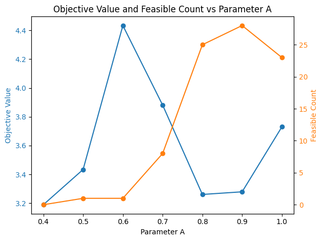
ax1.set_xlabel("Parameter A")
ax1.set_ylabel("Objective Value", color="tab:blue")
ax1.plot(table["parameter"]["A"], table["sampleset_0"]["obj_mean"], "-o", color="tab:blue")
ax1.tick_params(axis="y", labelcolor="tab:blue")

# Second y-axis for feasible count
ax2 = ax1.twinx()
ax2.set_ylabel("Feasible Count", color="tab:orange")
ax2.plot(table["parameter"]["A"], table["sampleset_0"]["feasible"], "-o", color="tab:orange")
ax2.tick_params(axis="y", labelcolor="tab:orange")

plt.title("Objective Value and Feasible Count vs Parameter A")
fig.tight_layout()