MIPソルバーの時間制限依存性に関する数値実験#
ここではOMMXでサポートされているPySCIPOptを用い、MIPソルバーの時間制限依存性に関する数値実験を行いましょう。 MINTOはOMMXメッセージをネイティブにサポートしているため、OMMXを通して数値実験をスムーズに行うことができます。
import minto
import ommx_pyscipopt_adapter as scip_ad
from ommx.dataset import miplib2017
ベンチマークターゲットとして、miplib2017からインスタンスを取得しましょう。
ommx.datasetを用いれば、簡単に取得することができます。
instance_name = "reblock115"
instance = miplib2017(instance_name)
ommx_pyscipopt_adapterを用いてommx.v1.InstanceをPySCIPOptのモデルに変換し、制限値/時間パラメータを変化させながら実験を行います。
ommxインスタンスと解は、MINTOの.log_*メソッドを用いて保存できます。
この数値実験では単一のインスタンスを使用するため、withブロックの外にあるexperiment空間に保存します。
制限時間ごとに解は変化するため、withブロック内(run空間内)に保存されます。
timelimit_list = [0.1, 0.5, 1, 2]


experiment = minto.Experiment(auto_saving=False)

experiment.log_global_instance(instance_name, instance)
adapter = scip_ad.OMMXPySCIPOptAdapter(instance)
scip_model = adapter.solver_input

for timelimit in timelimit_list:
    with experiment.run() as run:
        run.log_parameter("timelimit", timelimit)

        # Solve by SCIP
        scip_model.setParam("limits/time", timelimit)
        scip_model.optimize()
        solution = adapter.decode(scip_model)

        run.log_solution("scip", solution)
[2025-08-05 09:46:40] 🚀 Starting experiment '7e3c433d'
[2025-08-05 09:46:40]   ├─ 📊 Environment: OS: Darwin 24.5.0, CPU: Apple M2 (8 cores), Memory: 24.0 GB, Python: 3.11.11
[2025-08-05 09:46:40]   ├─ 📊 Environment Information
[2025-08-05 09:46:40]       ├─ OS: Darwin 24.5.0
[2025-08-05 09:46:40]       ├─ Platform: macOS-15.5-arm64-arm-64bit
[2025-08-05 09:46:40]       ├─ CPU: Apple M2 (8 cores)
[2025-08-05 09:46:40]       ├─ Memory: 24.0 GB
[2025-08-05 09:46:40]       ├─ Architecture: arm64
[2025-08-05 09:46:40]       ├─ Python: 3.11.11
[2025-08-05 09:46:40]       ├─ Virtual Environment: /Users/yuyamashiro/workspace/minto/.venv
[2025-08-05 09:46:40]       ├─ Key Package Versions:
[2025-08-05 09:46:40]   ├─ 🏃 Created run #0
[2025-08-05 09:46:40]       ├─ 📝 Parameter: timelimit = 0.1
[2025-08-05 09:46:40]       ├─ 🎯 Solution 'scip': objective: 0.000, feasible: True
[2025-08-05 09:46:40]   ├─ ✅ Run #0 completed (0.1s)
[2025-08-05 09:46:40]   ├─ 🏃 Created run #1
[2025-08-05 09:46:40]       ├─ 📝 Parameter: timelimit = 0.5
[2025-08-05 09:46:41]       ├─ 🎯 Solution 'scip': objective: -28241914.988, feasible: True
[2025-08-05 09:46:41]   ├─ ✅ Run #1 completed (0.4s)
[2025-08-05 09:46:41]   ├─ 🏃 Created run #2
[2025-08-05 09:46:41]       ├─ 📝 Parameter: timelimit = 1
[2025-08-05 09:46:41]       ├─ 🎯 Solution 'scip': objective: -28241914.988, feasible: True
[2025-08-05 09:46:41]   ├─ ✅ Run #2 completed (0.5s)
[2025-08-05 09:46:41]   ├─ 🏃 Created run #3
[2025-08-05 09:46:41]       ├─ 📝 Parameter: timelimit = 2
[2025-08-05 09:46:42]       ├─ 🎯 Solution 'scip': objective: -28241914.988, feasible: True
[2025-08-05 09:46:42]   ├─ ✅ Run #3 completed (1.0s)
.get_run_tableメソッドを用いてommx.Solutionをpandas.DataFrameに変換すると、解の主要な情報のみが表示されます。
実際の解オブジェクトにアクセスしたい場合は、experiment.dataspaces.run_datastores[run_id].solutionsから参照することができます。
runs_table = experiment.get_run_table()
runs_table
| solution_scip | parameter | metadata | |||||||
|---|---|---|---|---|---|---|---|---|---|
| objective | feasible | optimality | relaxation | start | name | timelimit | run_id | elapsed_time | |
| run_id | |||||||||
| 0 | 0.000000e+00 | True | 0 | 0 | None | scip | 0.1 | 0 | 0.110397 |
| 1 | -2.824191e+07 | True | 0 | 0 | None | scip | 0.5 | 1 | 0.410168 |
| 2 | -2.824191e+07 | True | 0 | 0 | None | scip | 1.0 | 2 | 0.506859 |
| 3 | -2.824191e+07 | True | 0 | 0 | None | scip | 2.0 | 3 | 1.008944 |
import matplotlib.pyplot as plt
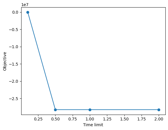
x = runs_table["parameter", "timelimit"]
y = runs_table["solution_scip", "objective"]
plt.plot(x, y, "o-")
plt.xlabel("Time limit")
plt.ylabel("Objective")
plt.show()
MINTOはネイティブにOMMXをサポートしているため、pandas.DataFrameに表示されるときは、主要な量のみが表示されます。 このため、統計分析を簡単に実行することができます。