QUBOのハイパーパラメータサーチ

ここでは、QUMOモデルのハイパーパラメータ空間を探索するために、MINTOがどのように使えるかを簡単な例を通して説明します。 この例では、2次割当定式化を用いて巡回セールスマン問題を扱います。 巡回セールスマン問題についての詳細は、ぜひ他のリソースを参照ください。

import minto
import matplotlib.pyplot as plt
import jijmodeling as jm

import minto.problems.tsp

tsp = minto.problems.tsp.QuadTSP()
tsp_problem = tsp.problem()

n = 8
tsp_data = tsp.data(n=n)

tsp_problem

\[\begin{split}\begin{array}{cccc}\text{Problem:} & \text{QuadTSP} & & \\& & \min \quad \displaystyle \sum_{i = 0}^{n - 1} \sum_{j = 0}^{n - 1} d_{i, j} \cdot \sum_{t = 0}^{n - 1} x_{i, t} \cdot x_{j, \left(t + 1\right) \bmod n} & \\\text{{s.t.}} & & & \\ & \text{one-city} & \displaystyle \sum_{\ast_{1} = 0}^{n - 1} x_{i, \ast_{1}} = 1 & \forall i \in \left\{0,\ldots,n - 1\right\} \\ & \text{one-time} & \displaystyle \sum_{\ast_{0} = 0}^{n - 1} x_{\ast_{0}, t} = 1 & \forall t \in \left\{0,\ldots,n - 1\right\} \\\text{{where}} & & & \\& x & 2\text{-dim binary variable}\\\end{array}\end{split}\]

interpreter = jm.Interpreter(tsp_data)
instance = interpreter.eval_problem(tsp_problem)

QUBO formulation

\[ E(x; A) = \sum_{i=0}^{n-1} \sum_{j=0}^{n-1} d_{ij} \sum_{t=0}^{n-1} x_{it} x_{j, (t+1)\mod n} + A \left[ \sum_i \left(\sum_{t} x_{i, t} - 1\right)^2 + \sum_t \left(\sum_{i} x_{i, t} - 1\right)^2 \right] \]

The parameter \(A\) is a hyperparameter that controls the strength of the constraints.

In OMMX, we can tune this parameter using the .to_qubo(uniform_penalty_weight=...) method and argument uniform_penalty_weight to set the value of \(A\).

import ommx_openjij_adapter as oj_ad

parameter_values = [0.4, 0.5, 0.6, 0.7, 0.8, 0.9, 1.0]

experiment = minto.Experiment(auto_saving=False, verbose_logging=False)
for A in parameter_values:
    with experiment.run() as run:
        ox_sampleset = oj_ad.OMMXOpenJijSAAdapter.sample(instance, uniform_penalty_weight=A, num_reads=30)
        run.log_sampleset(ox_sampleset)
        run.log_parameter("A", A)

table = experiment.get_run_table()
table

	sampleset_0							parameter	metadata
	num_samples	obj_mean	obj_std	obj_min	obj_max	feasible	name	A	run_id	elapsed_time
run_id
0	30	3.353026	0.499013	2.355019	4.268100	0	0	0.4	0	0.042427
1	30	3.383542	0.700817	2.340510	4.839428	0	0	0.5	1	0.034157
2	30	6.323973	1.107701	4.669342	8.462845	0	0	0.6	2	0.036005
3	30	2.939773	0.576959	2.220747	4.255948	16	0	0.7	3	0.028858
4	30	2.536650	0.234261	2.220747	3.052677	29	0	0.8	4	0.028297
5	30	2.686100	0.275722	2.220747	3.506836	30	0	0.9	5	0.021842
6	30	2.722490	0.341214	2.220747	3.609280	30	0	1.0	6	0.022454

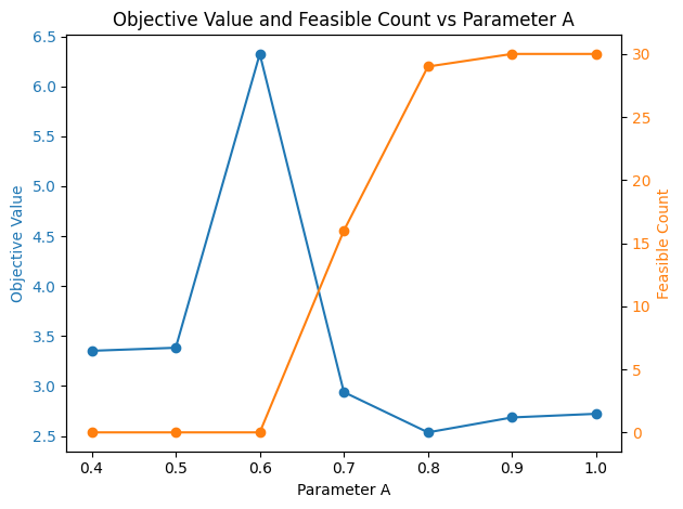
fig, ax1 = plt.subplots()

# First y-axis for objective value
ax1.set_xlabel("Parameter A")
ax1.set_ylabel("Objective Value", color="tab:blue")
ax1.plot(table["parameter"]["A"], table["sampleset_0"]["obj_mean"], "-o", color="tab:blue")
ax1.tick_params(axis="y", labelcolor="tab:blue")

# Second y-axis for feasible count
ax2 = ax1.twinx()
ax2.set_ylabel("Feasible Count", color="tab:orange")
ax2.plot(table["parameter"]["A"], table["sampleset_0"]["feasible"], "-o", color="tab:orange")
ax2.tick_params(axis="y", labelcolor="tab:orange")

plt.title("Objective Value and Feasible Count vs Parameter A")
fig.tight_layout()