Performance Comparison of MIP Solver Formulations for Capacitated VRP

Performance Comparison of MIP Solver Formulations for Capacitated VRP#

This notebook compares the performance of different formulations for the Capacitated Vehicle Routing Problem (CVRP) using MIP solvers. CVRP is a variant of the Vehicle Routing Problem (VRP) where each customer has a demand and vehicles have capacity constraints. CVRP generalizes VRP, which can be considered as a special case of CVRP.

We implement each model using JijModeling, manage optimization results with MINTO, and solve the models using SCIP. Finally, we compare the performance of each model.

MTZ formulation and Flow formulation#

For CVRP, there are two major formulations: MTZ formulation (also called potential formulation) and Flow formulation.

About Each Formulation#

MTZ formulation and Flow formulation differ in how they track cumulative demand. MTZ formulation tracks cumulative demand at each customer node, while Flow formulation tracks flow amount on each edge. The concept is illustrated in the figure below:

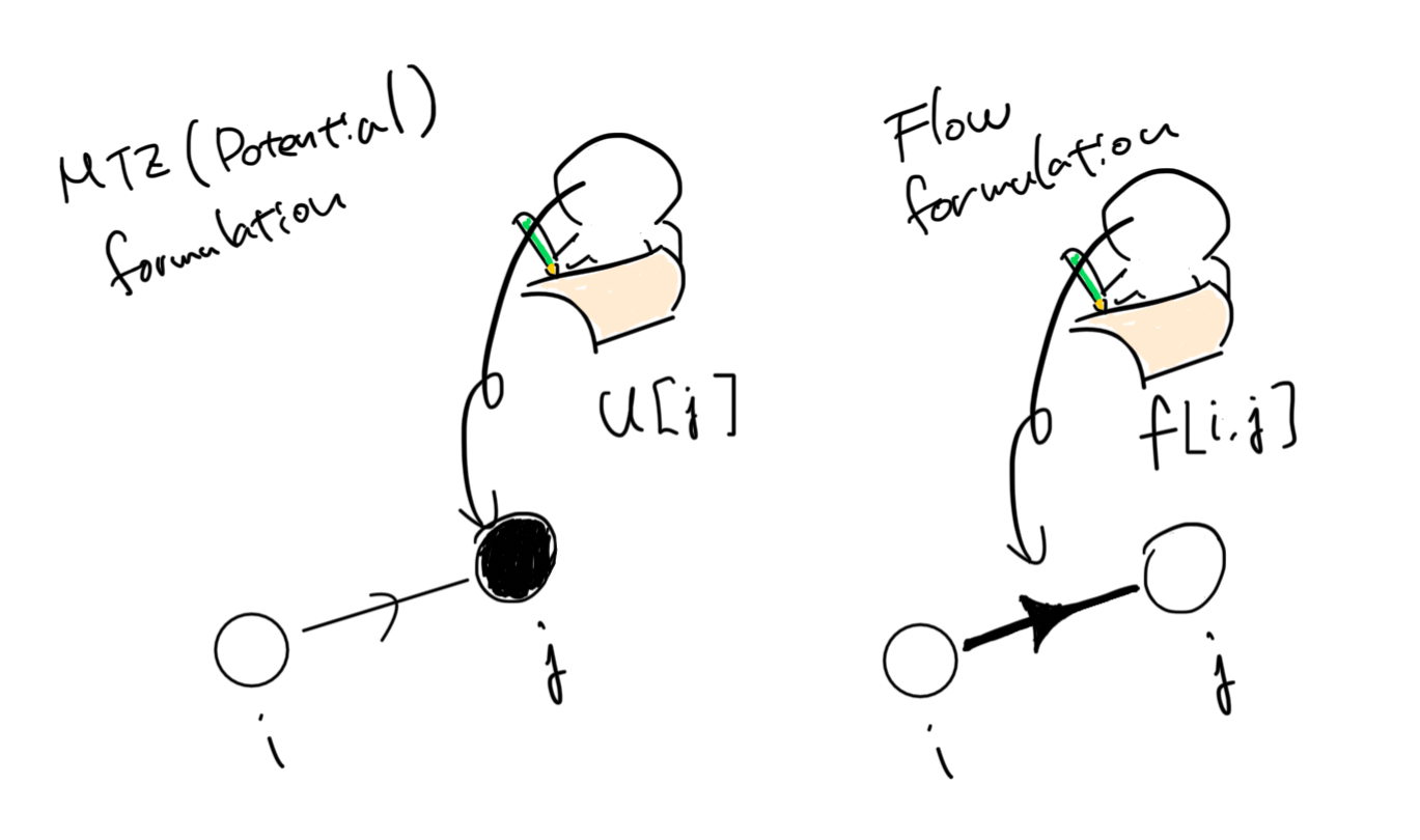cvrp_mtz_flow Illustration of u and f variables in MTZ and Flow formulations. In MTZ formulation, u records the vehicle load at each node. In Flow formulation, f records the available capacity of vehicles on each edge.

MTZ (Miller-Tucker-Zemlin) Formulation: MTZ formulation introduces continuous variables representing cumulative demand at each customer node to express subtour elimination constraints. This method has relatively fewer variables and a simpler model but weaker LP relaxation.
Flow Formulation: Flow formulation introduces continuous variables representing flow amount on each edge and uses flow conservation laws to express subtour elimination constraints. This method has more variables but stronger LP relaxation.

Let’s implement these two formulations and compare their performance.

Common Parts of CVRP Formulation#

Let’s first implement the parts common to both models.

import minto
import jijmodeling as jm
from minto.problems.cvrp import CVRPMTZ, CVRPFlow

MTZ formulation#

CVRPMTZ().problem()

\[\begin{split}\begin{array}{cccc}\text{Problem:} & \text{CVRPMTZ} & & \\& & \min \quad \displaystyle \sum_{i = 0}^{n - 1} \sum_{j = 0}^{n - 1} c_{i, j} \cdot x_{i, j} & \\\text{{s.t.}} & & & \\ & \text{in} & \displaystyle \sum_{\ast_{1} = 0}^{n - 1} x_{i, \ast_{1}} = 1 & \forall i \in \left\{i \in \left\{0,\ldots,n - 1\right\} \mid i > 0 \right\} \\ & \text{no loop} & \displaystyle x_{i, i} = 0 & \forall i \in \left\{0,\ldots,n - 1\right\} \\ & \text{out} & \displaystyle \sum_{\ast_{0} = 0}^{n - 1} x_{\ast_{0}, i} = 1 & \forall i \in \left\{i \in \left\{0,\ldots,n - 1\right\} \mid i > 0 \right\} \\ & \text{potiantial} & \displaystyle u_{i} + D_{j} - Q \cdot \left(- x_{i, j} + 1\right) + \left(Q - D_{i} - D_{j}\right) \cdot x_{j, i} \leq u_{j} & \forall i \in \left\{0,\ldots,n - 1\right\} \forall j \in \left\{j \in \left\{0,\ldots,n - 1\right\} \mid j \neq 0 \right\} \\\text{{where}} & & & \\& x & 2\text{-dim binary variable}& \text{use edge or not}\\& u & 1\text{-dim continuous variable}& \text{cumulative demand}\\ & & \text{lower bound: }D & \\ & & \text{upper bound: }Q & \\\end{array}\end{split}\]

Flow formulation#

CVRPFlow().problem()

\[\begin{split}\begin{array}{cccc}\text{Problem:} & \text{CVRPFlow} & & \\& & \min \quad \displaystyle \sum_{i = 0}^{n - 1} \sum_{j = 0}^{n - 1} c_{i, j} \cdot x_{i, j} & \\\text{{s.t.}} & & & \\ & \text{flow} & \displaystyle \sum_{j = 0}^{n - 1} f_{j, i} - \sum_{j = 0}^{n - 1} f_{i, j} = D_{i} & \forall i \in \left\{i \in \left\{0,\ldots,n - 1\right\} \mid i > 0 \right\} \\ & \text{flow cap} & \displaystyle f_{i, j} \leq \left(Q - D_{i}\right) \cdot x_{i, j} & \forall i \in \left\{0,\ldots,n - 1\right\} \forall j \in \left\{0,\ldots,n - 1\right\} \\ & \text{in} & \displaystyle \sum_{\ast_{1} = 0}^{n - 1} x_{i, \ast_{1}} = 1 & \forall i \in \left\{i \in \left\{0,\ldots,n - 1\right\} \mid i > 0 \right\} \\ & \text{no loop} & \displaystyle x_{i, i} = 0 & \forall i \in \left\{0,\ldots,n - 1\right\} \\ & \text{out} & \displaystyle \sum_{\ast_{0} = 0}^{n - 1} x_{\ast_{0}, i} = 1 & \forall i \in \left\{i \in \left\{0,\ldots,n - 1\right\} \mid i > 0 \right\} \\\text{{where}} & & & \\& x & 2\text{-dim binary variable}& \text{use edge or not}\\& f & 2\text{-dim continuous variable}& \text{cumulative demand}\\ & & \text{lower bound: }0 & \\ & & \text{upper bound: }Q & \\\end{array}\end{split}\]

Random CVRP Instance Generation#

We generate a random CVRP instance to test the models.

import matplotlib.pyplot as plt

n = 10
instance_data = CVRPFlow().random_data(n)
xy = instance_data['xy']

Performance Comparison#

We compare the performance of the two formulations using the random CVRP instance. The JijModeling implementation is converted to PySCIPOpt using ommx_pyscipopt_adapter and solved with SCIP. Results are logged using MINTO.

When logging using .log_instance, we assign names to each model to make later comparison easier.

For this tutorial we set auto_saving=False, but in practice it is recommended to use auto_saving=True for automatic log saving.

import time
import ommx_pyscipopt_adapter as scip_ad

exp = minto.Experiment("cvrp", auto_saving=False)

nlist = [8, 9, 10, 11, 12, 13]
for n in nlist:
    print(f"{n=}")
    with exp.run():
        instance_data = CVRPFlow().random_data(n)
        exp.log_parameter("n", n)
        intepreter = jm.Interpreter(instance_data)

        # MTZ model
        mtz_instance = intepreter.eval_problem(CVRPMTZ().problem())
        exp.log_instance("mtz", mtz_instance)
    
        adapter = scip_ad.OMMXPySCIPOptAdapter(mtz_instance)
        scip_model = adapter.solver_input

        start = time.time()
        scip_model.optimize()
        scip_model.getStatus()
        elpsed_time = time.time() - start

        exp.log_parameter("mtz_time", elpsed_time)

        mtz_solution = adapter.decode(scip_model)
        exp.log_solution("mtz", mtz_solution)

        # Flow model
        intepreter = jm.Interpreter(instance_data)
        flow_instance = intepreter.eval_problem(CVRPFlow().problem())
        exp.log_instance("flow", flow_instance)
    
        adapter = scip_ad.OMMXPySCIPOptAdapter(flow_instance)
        scip_model = adapter.solver_input

        start = time.time()
        scip_model.optimize()
        scip_model.getStatus()
        elpsed_time = time.time() - start

        exp.log_parameter("flow_time", elpsed_time)

        flow_solution = adapter.decode(scip_model)
        exp.log_solution("flow", flow_solution)

n=8
n=9
n=10
n=11
n=12
n=13

exp.get_run_table()

	instance_mtz							instance_flow			...	solution_flow					parameter			metadata
	num_vars	num_binary	num_integer	num_continuous	num_cons	title	name	num_vars	num_binary	num_integer	...	feasible	optimality	relaxation	start	name	n	mtz_time	flow_time	run_id	elapsed_time
run_id
0	90	81	0	9	None	None	mtz	162	81	0	...	True	1	0	None	flow	8	0.463605	0.524607	0	1.559064
1	110	100	0	10	None	None	mtz	200	100	0	...	True	1	0	None	flow	9	1.925011	2.292580	1	4.838226
2	132	121	0	11	None	None	mtz	242	121	0	...	True	1	0	None	flow	10	5.972111	2.976185	2	9.516440
3	156	144	0	12	None	None	mtz	288	144	0	...	True	1	0	None	flow	11	2.741986	0.900541	3	4.211383
4	182	169	0	13	None	None	mtz	338	169	0	...	True	1	0	None	flow	12	1559.416442	66.239141	4	1626.341933
5	210	196	0	14	None	None	mtz	392	196	0	...	True	1	0	None	flow	13	66.974998	42.733377	5	110.349438

6 rows × 31 columns

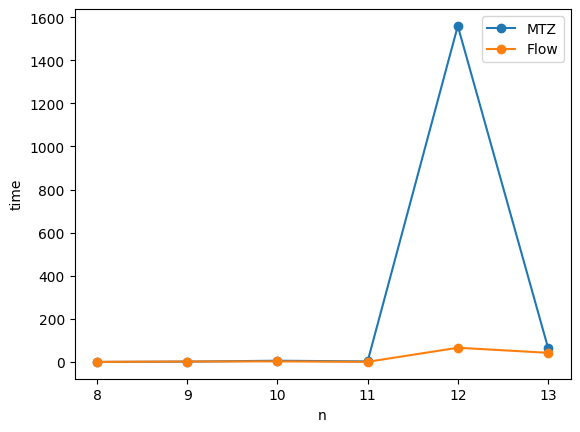
param_table = exp.get_run_table()['parameter']
plt.plot(param_table['n'], param_table['mtz_time'], "-o", label="MTZ")
plt.plot(param_table['n'], param_table['flow_time'], "-o", label="Flow")
plt.legend()
plt.xlabel("n")
plt.ylabel("time")
plt.show()

../_images/f0084c55360458f4f979cfda131b772aeb9bdde4a42bb29065df23a4ca150c7e.png

Summary#

In this notebook, we implemented MTZ and Flow formulations for the Capacitated Vehicle Routing Problem (CVRP) and compared their performance using a random CVRP instance. We found that the Flow formulation is faster than the MTZ formulation for the given instance.

It is interesting to note that despite having more variables, the Flow formulation performs better. This serves as a good example of how the effectiveness of branch-and-bound methods can vary depending on the constraint conditions and how easy they are to solve.

However, the performance may vary depending on the instance characteristics. For example, different vehicle capacities could lead to significantly different results. Additionally, there are strengthened versions of the MTZ formulation available.

Feel free to experiment with different instance generation methods and strengthened versions of the MTZ formulation.