Numerical Experiments on Time Limit Dependency of MIP Solver

In this notebook, we will conduct numerical experiments on the time limit dependency of MIP solvers using PySCIPOpt, which is supported by OMMX. MINTO natively supports OMMX Message, allowing us to smoothly perform numerical experiments through OMMX. Let’s give it a try.

import minto
import ommx_pyscipopt_adapter as scip_ad
from ommx.dataset import miplib2017

In this tutorial, we will pick up an instance from miplib2017 as a benchmark target. We can easily obtain miplib2017 instances using ommx.dataset.

instance_name = "reblock115"
instance = miplib2017(instance_name)

Using the ommx_pyscipopt_adapter, we convert ommx.v1.Instance to PySCIPOpt’s Model and conduct experiments by varying the limits/time parameter.

The ommx instance and solution can be saved using MINTO’s .log_* methods. Since we’re using a single instance that doesn’t change throughout this numerical experiment, we store it in the experiment space outside the with block. Solutions are saved within the with block (in the run space) since they vary for each time limit.

timelimit_list = [0.1, 0.5, 1, 2]


experiment = minto.Experiment(auto_saving=False)

experiment.log_instance(instance_name, instance)
adapter = scip_ad.OMMXPySCIPOptAdapter(instance)
scip_model = adapter.solver_input

for timelimit in timelimit_list:
    with experiment.run():
        experiment.log_parameter("timelimit", timelimit)

        # Solve by SCIP
        scip_model.setParam("limits/time", timelimit)
        scip_model.optimize()
        solution = adapter.decode(scip_model)

        experiment.log_solution('scip', solution)

When converting ommx.Solution to pandas.DataFrame using the .get_run_table method, only the main information of the solution is displayed. If you want to access the actual solution objects, you can reference them from experiment.dataspaces.run_datastores[run_id].solutions.

runs_table = experiment.get_run_table()
runs_table

	solution_scip						parameter	metadata
	objective	feasible	optimality	relaxation	start	name	timelimit	run_id	elapsed_time
run_id
0	0.000000e+00	True	0	0	None	scip	0.1	0	0.106656
1	-2.824191e+07	True	0	0	None	scip	0.5	1	0.407615
2	-2.824191e+07	True	0	0	None	scip	1.0	2	0.505631
3	-2.824191e+07	True	0	0	None	scip	2.0	3	1.006043

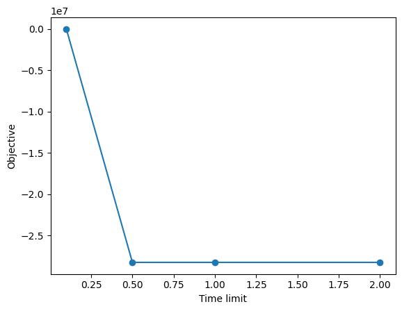
import matplotlib.pyplot as plt

x = runs_table['parameter', 'timelimit']
y = runs_table['solution_scip', 'objective']
plt.plot(x, y, 'o-')
plt.xlabel('Time limit')
plt.ylabel('Objective')
plt.show()

As MINTO natively supports OMMX, only the main quantities are displayed when shown in a pandas.DataFrame, making it easy to perform statistical analysis.