Solving Optimization Problems with OMMX Adapter#
OMMX provides OMMX Adapter software to enable interoperability with existing mathematical optimization tools. By using OMMX Adapter, you can convert optimization problems expressed in OMMX schemas into formats acceptable to other optimization tools, and convert the resulting data from those tools back into OMMX schemas.
Here, we introduce how to solve a 0-1 Knapsack Problem via OMMX PySCIPOpt Adapter.
Installing the Required Libraries#
First, install OMMX PySCIPOpt Adapter with:
pip install ommx-pyscipopt-adapter
Two Steps for Running the Optimization#
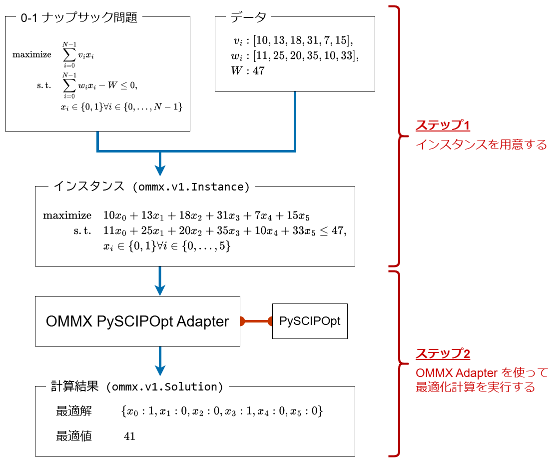
Fig. 4 Flow for solving 0-1 Knapsack Problem with OMMX PySCIPOpt Adapter.#
To solve the 0-1 Knapsack Problem through the OMMX PySCIPOpt Adapter, follow these two steps:
Prepare the 0-1 Knapsack problem instance.
Run the optimization via OMMX Adapter.
In Step 1, we create an ommx.v1.Instance object defined in the OMMX Message Instance schema. There are several ways to generate this object, but in this guide, we’ll illustrate how to write it directly using the OMMX Python SDK.
Tip
There are four ways to prepare an ommx.v1.Instance object:
Write
ommx.v1.Instancedirectly with the OMMX Python SDK.Convert an MPS file to
ommx.v1.Instanceusing the OMMX Python SDK.Convert a problem instance from a different optimization tool into
ommx.v1.Instanceusing an OMMX Adapter.Export
ommx.v1.Instancefrom JijModeling.
In Step 2, we convert ommx.v1.Instance into a PySCIPOpt Model object and run optimization with SCIP. The result is obtained as an ommx.v1.Solution object defined by the OMMX Message Solution schema.
Step 1: Preparing a 0-1 Knapsack Problem Instance#
The 0-1 Knapsack problem is formulated as:
Here, we set the following data as parameters for this mathematical model:
# Data for 0-1 Knapsack Problem
v = [10, 13, 18, 31, 7, 15]   # Values of each item
w = [11, 25, 20, 35, 10, 33] # Weights of each item
W = 47  # Capacity of the knapsack
N = len(v)  # Total number of items
Based on this mathematical model and data, the code for describing the problem instance using the OMMX Python SDK is as follows:
from ommx.v1 import Instance, DecisionVariable

# Define decision variables
x = [
    # Define binary variable x_i
    DecisionVariable.binary(
        # Specify the ID of the decision variable
        id=i,
        # Specify the name of the decision variable
        name="x",
        # Specify the subscript of the decision variable
        subscripts=[i],
    )
    # Prepare binary variables for the number of items
    for i in range(N)
]

# Define the objective function
objective = sum(v[i] * x[i] for i in range(N))

# Define the constraint
constraint = (sum(w[i] * x[i] for i in range(N)) <= W).add_name("Weight limit")

# Create an instance
instance = Instance.from_components(
    # Register all decision variables included in the instance
    decision_variables=x,
    # Register the objective function
    objective=objective,
    # Register all constraints
    constraints=[constraint],
    # Specify that it is a maximization problem
    sense=Instance.MAXIMIZE,
)
Step 2: Running Optimization with OMMX Adapter#
To optimize the instance prepared in Step 1, we run the optimization calculation via the OMMX PySCIPOpt Adapter as follows:
from ommx_pyscipopt_adapter import OMMXPySCIPOptAdapter

# Obtain an ommx.v1.Solution object through a PySCIPOpt model.
solution = OMMXPySCIPOptAdapter.solve(instance)
The variable solution here is an ommx.v1.Solution object that contains the results of the optimization calculation by SCIP.
Analyzing the Results#
From the calculation results obtained in Step 2, we can check and analyze:
The optimal solution (the way to select items that maximizes the total value of items)
The optimal value (the highest total value of items)
The constraints (the margin of the total weight of items against the weight limit)
To do this, we use the properties implemented in the ommx.v1.Solution class.
Analyzing the Optimal Solution#
The decision_variables_df property returns a pandas.DataFrame object containing information on each variable, such as ID, type, name, and value:
solution.decision_variables_df
| kind | lower | upper | name | subscripts | description | substituted_value | value | |
|---|---|---|---|---|---|---|---|---|
| id | ||||||||
| 0 | Binary | 0.0 | 1.0 | x | [0] | <NA> | <NA> | 1.0 |
| 1 | Binary | 0.0 | 1.0 | x | [1] | <NA> | <NA> | 0.0 |
| 2 | Binary | 0.0 | 1.0 | x | [2] | <NA> | <NA> | 0.0 |
| 3 | Binary | 0.0 | 1.0 | x | [3] | <NA> | <NA> | 1.0 |
| 4 | Binary | 0.0 | 1.0 | x | [4] | <NA> | <NA> | 0.0 |
| 5 | Binary | 0.0 | 1.0 | x | [5] | <NA> | <NA> | 0.0 |
Using this pandas.DataFrame object, you can easily create a table in pandas that shows, for example, “whether to put items in the knapsack”:
import pandas as pd

df = solution.decision_variables_df
pd.DataFrame.from_dict(
    {
        "Item number": df.index,
        "Include in knapsack?": df["value"].apply(lambda x: "Include" if x == 1.0 else "Exclude"),
    }
)
| Item number | Include in knapsack? | |
|---|---|---|
| id | ||
| 0 | 0 | Include |
| 1 | 1 | Exclude |
| 2 | 2 | Exclude |
| 3 | 3 | Include |
| 4 | 4 | Exclude |
| 5 | 5 | Exclude |
From this analysis result, we can see that choosing items 0 and 3 maximizes the total value while satisfying the knapsack’s weight constraint.
Analyzing the Optimal Value#
The objective property stores the optimal value. In this case, it should be the sum of the values of items 0 and 3:
import numpy as np
# The expected value is the sum of the values of items 0 and 3
expected = v[0] + v[3]
assert np.isclose(solution.objective, expected)
Analyzing Constraints#
The constraints_df property returns a pandas.DataFrame object that includes details about each constraint’s equality or inequality, its left-hand-side value ("value"), name, and more:
solution.constraints_df
| equality | value | used_ids | name | subscripts | description | dual_variable | removed_reason | |
|---|---|---|---|---|---|---|---|---|
| id | ||||||||
| 0 | <=0 | -1.0 | {0, 1, 2, 3, 4, 5} | Weight limit | [] | <NA> | <NA> | <NA> |
Specifically, the "value" is helpful for understanding how much slack remains in each constraint. In this case, item 0 has weight \(w_0 = 11\), item 3 has weight \(w_3 = 35\), and the knapsack’s capacity \(W\) is \(47\). Therefore, for the weight constraint
the left-hand side “value” is \(-1\), indicating there is exactly \(1\) unit of slack under the capacity.