Solve with multiple adapters and compare the results

Since the OMMX Adapter provides a unified API, you can solve the same problem using multiple solvers and compare the results. Let’s consider a simple knapsack problem as an example:

\[\begin{split} \begin{align*} \mathrm{maximize} \quad & \sum_{i=0}^{N-1} v_i x_i \\ \mathrm{s.t.} \quad & \sum_{i=0}^{n-1} w_i x_i - W \leq 0, \\ & x_{i} \in \{ 0, 1\} \end{align*} \end{split}\]

from ommx.v1 import Instance, DecisionVariable

v = [10, 13, 18, 31, 7, 15]
w = [11, 25, 20, 35, 10, 33]
W = 47
N = len(v)

x = [
    DecisionVariable.binary(
        id=i,
        name="x",
        subscripts=[i],
    )
    for i in range(N)
]
instance = Instance.from_components(
    decision_variables=x,
    objective=sum(v[i] * x[i] for i in range(N)),
    constraints=[sum(w[i] * x[i] for i in range(N)) - W <= 0],
    sense=Instance.MAXIMIZE,
)

Solve with multiple adapters

Here, we will use the following OSS solvers with corresponding adapters, which are developed as a part of OMMX Python SDK:

Package name	PyPI	Backend
ommx-python-mip-adapter		CBC via Python-MIP
ommx-pyscipopt-adapter		SCIP via PySCIPOpt
ommx-highs-adapter		HiGHS

For non-OSS solvers, the following adapters also developed as separated repositories:

Package name	PyPI	Backend
ommx-gurobipy-adapter		Gurobi
ommx-fixstars-amplify-adapter		Fixstars Amplify

Here, let’s solve the knapsack problem with OSS solvers, Highs, Python-MIP (CBC), and SCIP.

from ommx_python_mip_adapter import OMMXPythonMIPAdapter
from ommx_pyscipopt_adapter  import OMMXPySCIPOptAdapter
from ommx_highs_adapter      import OMMXHighsAdapter

# List of adapters to use
adapters = {
    "highs": OMMXHighsAdapter,
    "cbc": OMMXPythonMIPAdapter,
    "scip": OMMXPySCIPOptAdapter,
}

# Solve the problem using each adapter
solutions = {
    name: adapter.solve(instance) for name, adapter in adapters.items()
}

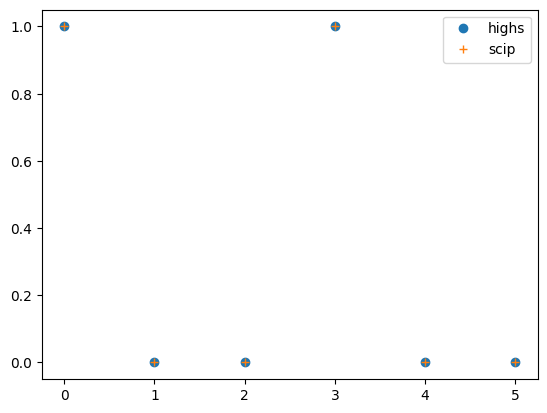
Compare the results

Since this knapsack problem is simple, all solvers will find the optimal solution.

from matplotlib import pyplot as plt

marks = {
    "highs": "o",
    "cbc": "x",
    "scip": "+",
}

for name, solution in solutions.items():
    x = solution.extract_decision_variables("x")
    subscripts = [key[0] for key in x.keys()]
    plt.plot(subscripts, x.values(), marks[name], label=name)

plt.legend()

<matplotlib.legend.Legend at 0x7f4273d5ca90>

It would be convenient to concatenate the pandas.DataFrame obtained with decision_variables when analyzing the results of multiple solvers.

import pandas

decision_variables = pandas.concat([
    solution.decision_variables.assign(solver=solver)
    for solver, solution in solutions.items()
])
decision_variables

	kind	lower	upper	name	subscripts	description	substituted_value	value	solver
id
0	binary	0.0	1.0	x	[0]	<NA>	<NA>	1.0	highs
1	binary	0.0	1.0	x	[1]	<NA>	<NA>	0.0	highs
2	binary	0.0	1.0	x	[2]	<NA>	<NA>	0.0	highs
3	binary	0.0	1.0	x	[3]	<NA>	<NA>	1.0	highs
4	binary	0.0	1.0	x	[4]	<NA>	<NA>	0.0	highs
5	binary	0.0	1.0	x	[5]	<NA>	<NA>	0.0	highs
0	binary	0.0	1.0	x	[0]	<NA>	<NA>	1.0	cbc
1	binary	0.0	1.0	x	[1]	<NA>	<NA>	0.0	cbc
2	binary	0.0	1.0	x	[2]	<NA>	<NA>	0.0	cbc
3	binary	0.0	1.0	x	[3]	<NA>	<NA>	1.0	cbc
4	binary	0.0	1.0	x	[4]	<NA>	<NA>	0.0	cbc
5	binary	0.0	1.0	x	[5]	<NA>	<NA>	0.0	cbc
0	binary	0.0	1.0	x	[0]	<NA>	<NA>	1.0	scip
1	binary	0.0	1.0	x	[1]	<NA>	<NA>	0.0	scip
2	binary	0.0	1.0	x	[2]	<NA>	<NA>	0.0	scip
3	binary	0.0	1.0	x	[3]	<NA>	<NA>	1.0	scip
4	binary	0.0	1.0	x	[4]	<NA>	<NA>	0.0	scip
5	binary	0.0	1.0	x	[5]	<NA>	<NA>	0.0	scip