Sampling from QUBO with OMMX Adapter

Here, we explain how to convert a problem to QUBO and perform sampling using the Traveling Salesman Problem as an example.

Fig. 5 Illustration of a man in a suit

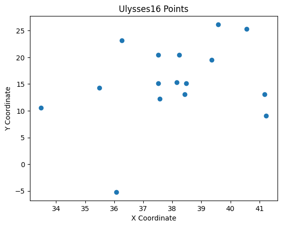
The Traveling Salesman Problem (TSP) is about finding a route for a salesman to visit multiple cities in sequence. Given the travel costs between cities, we seek to find the path that minimizes the total cost. Let’s consider the following city arrangement:

# From ulysses16.tsp in TSPLIB
ulysses16_points = [
    (38.24, 20.42),
    (39.57, 26.15),
    (40.56, 25.32),
    (36.26, 23.12),
    (33.48, 10.54),
    (37.56, 12.19),
    (38.42, 13.11),
    (37.52, 20.44),
    (41.23, 9.10),
    (41.17, 13.05),
    (36.08, -5.21),
    (38.47, 15.13),
    (38.15, 15.35),
    (37.51, 15.17),
    (35.49, 14.32),
    (39.36, 19.56),
]

Let’s plot the locations of the cities.

%matplotlib inline
from matplotlib import pyplot as plt

x_coords, y_coords = zip(*ulysses16_points)
plt.scatter(x_coords, y_coords)
plt.xlabel('X Coordinate')
plt.ylabel('Y Coordinate')
plt.title('Ulysses16 Points')
plt.show()

Let’s consider distance as the cost. We’ll calculate the distance \(d(i, j)\) between city \(i\) and city \(j\).

def distance(x, y):
    return ((x[0] - y[0])**2 + (x[1] - y[1])**2)**0.5

# Number of cities
N = len(ulysses16_points)
# Distance between each pair of cities
d = [[distance(ulysses16_points[i], ulysses16_points[j]) for i in range(N)] for j in range(N)]

Using this, we can formulate TSP as follows. First, let’s represent whether we are at city \(i\) at time \(t\) with a binary variable \(x_{t, i}\). Then, we seek \(x_{t, i}\) that satisfies the following constraints. The distance traveled by the salesman is given by:

\[ \sum_{t=0}^{N-1} \sum_{i, j = 0}^{N-1} d(i, j) x_{t, i} x_{(t+1 \% N), j} \]

However, \(x_{t, i}\) cannot be chosen freely and must satisfy two constraints: at each time \(t\), the salesman can only be in one city, and each city must be visited exactly once:

\[ \sum_{i=0}^{N-1} x_{t, i} = 1, \quad \sum_{t=0}^{N-1} x_{t, i} = 1 \]

Combining these, TSP can be formulated as a constrained optimization problem:

\[\begin{split} \begin{align*} \min \quad & \sum_{t=0}^{N-1} \sum_{i, j = 0}^{N-1} d(i, j) x_{t, i} x_{(t+1 \% N), j} \\ \text{s.t.} \quad & \sum_{i=0}^{N-1} x_{t, i} = 1 \quad (\forall t = 0, \ldots, N-1) \\ \quad & \sum_{t=0}^{N-1} x_{t, i} = 1 \quad (\forall i = 0, \ldots, N-1) \end{align*} \end{split}\]

The corresponding ommx.v1.Instance can be created as follows:

from ommx.v1 import DecisionVariable, Instance

x = [[
        DecisionVariable.binary(
            i + N * t,  # Decision variable ID
            name="x",           # Name of the decision variable, used when extracting solutions
            subscripts=[t, i])  # Subscripts of the decision variable, used when extracting solutions
        for i in range(N)
    ]
    for t in range(N)
]

objective = sum(
    d[i][j] * x[t][i] * x[(t+1) % N][j]
    for i in range(N)
    for j in range(N)
    for t in range(N)
)
place_constraint = [
    (sum(x[t][i] for i in range(N)) == 1)
        .set_id(t)  # type: ignore
        .add_name("place")
        .add_subscripts([t])
    for t in range(N)
]
time_constraint = [
    (sum(x[t][i] for t in range(N)) == 1)
        .set_id(i + N)  # type: ignore
        .add_name("time")
        .add_subscripts([i])
    for i in range(N)
]

instance = Instance.from_components(
    decision_variables=[x[t][i] for i in range(N) for t in range(N)],
    objective=objective,
    constraints=place_constraint + time_constraint,
    sense=Instance.MINIMIZE
)

The variable names and subscripts added to DecisionVariable.binary during creation will be used later when interpreting the obtained samples.

Sampling with OpenJij

To sample the QUBO described by ommx.v1.Instance using OpenJij, use the ommx-openjij-adapter.

from ommx_openjij_adapter import OMMXOpenJijSAAdapter

sample_set = OMMXOpenJijSAAdapter.sample(instance, num_reads=16, uniform_penalty_weight=20.0)
sample_set.summary

	objective	feasible
sample_id
6	99.936405	True
2	100.122451	True
11	100.658428	True
12	103.871457	True
13	104.641484	True
9	112.343693	True
7	86.762146	False
15	92.088925	False
10	99.063975	False
3	99.151124	False
1	99.244552	False
0	105.292839	False
14	112.321550	False
4	113.798689	False
8	115.560848	False
5	122.694561	False

OMMXOpenJijSAAdapter.sample returns ommx.v1.SampleSet, which stores the evaluated objective function values and constraint violations in addition to the decision variable values of samples. The SampleSet.summary property is used to display summary information. feasible indicates the feasibility to the original problem before conversion to QUBO. This is calculated using the information stored in removed_constraints of the qubo instance.

To view the feasibility for each constraint, use the summary_with_constraints property.

sample_set.summary_with_constraints

	objective	feasible	place[0]	place[1]	place[2]	place[3]	place[4]	place[5]	place[6]	place[7]	...	time[6]	time[7]	time[8]	time[9]	time[10]	time[11]	time[12]	time[13]	time[14]	time[15]
sample_id
6	99.936405	True	True	True	True	True	True	True	True	True	...	True	True	True	True	True	True	True	True	True	True
2	100.122451	True	True	True	True	True	True	True	True	True	...	True	True	True	True	True	True	True	True	True	True
11	100.658428	True	True	True	True	True	True	True	True	True	...	True	True	True	True	True	True	True	True	True	True
12	103.871457	True	True	True	True	True	True	True	True	True	...	True	True	True	True	True	True	True	True	True	True
13	104.641484	True	True	True	True	True	True	True	True	True	...	True	True	True	True	True	True	True	True	True	True
9	112.343693	True	True	True	True	True	True	True	True	True	...	True	True	True	True	True	True	True	True	True	True
7	86.762146	False	True	True	True	True	True	True	True	True	...	True	True	True	True	False	True	True	True	True	True
15	92.088925	False	True	True	True	True	True	True	False	True	...	True	True	True	True	False	True	True	True	True	True
10	99.063975	False	True	True	True	True	True	True	True	True	...	True	True	True	True	False	True	True	True	True	True
3	99.151124	False	True	True	True	False	True	True	True	True	...	True	True	True	True	False	True	True	True	True	True
1	99.244552	False	False	True	True	True	True	True	True	True	...	True	True	True	True	False	True	True	True	True	True
0	105.292839	False	False	True	True	True	True	True	True	True	...	True	True	True	True	False	True	True	True	True	True
14	112.321550	False	True	True	True	True	True	True	True	True	...	True	True	True	True	False	True	True	True	True	True
4	113.798689	False	True	True	False	True	True	True	True	True	...	True	True	True	True	False	True	True	True	True	True
8	115.560848	False	True	True	True	True	True	True	True	True	...	True	True	True	True	False	True	True	True	True	True
5	122.694561	False	True	True	True	True	True	True	True	True	...	True	True	True	True	False	True	True	True	True	True

16 rows × 34 columns

For more detailed information, you can use the SampleSet.decision_variables and SampleSet.constraints properties.

sample_set.decision_variables_df.head(2)

	kind	lower	upper	name	subscripts	description	0	1	2	3	...	6	7	8	9	10	11	12	13	14	15
id
0	Binary	0.0	1.0	x	[0, 0]	None	0.0	0.0	1.0	0.0	...	0.0	0.0	0.0	0.0	0.0	0.0	0.0	0.0	0.0	0.0
1	Binary	0.0	1.0	x	[0, 1]	None	0.0	0.0	0.0	0.0	...	0.0	0.0	0.0	0.0	1.0	0.0	0.0	0.0	0.0	0.0

2 rows × 22 columns

sample_set.constraints_df.head(2)

	equality	used_ids	name	subscripts	description	removed_reason	value.0	value.1	value.2	value.3	...	feasible.6	feasible.7	feasible.8	feasible.9	feasible.10	feasible.11	feasible.12	feasible.13	feasible.14	feasible.15
id
0	=0	{0, 1, 2, 3, 4, 5, 6, 7, 8, 9, 10, 11, 12, 13,...	place	[0]	None	uniform_penalty_method	-1.0	-1.0	0.0	0.0	...	True	True	True	True	True	True	True	True	True	True
1	=0	{16, 17, 18, 19, 20, 21, 22, 23, 24, 25, 26, 2...	place	[1]	None	uniform_penalty_method	0.0	0.0	0.0	0.0	...	True	True	True	True	True	True	True	True	True	True

2 rows × 38 columns

To obtain the samples, use the SampleSet.extract_decision_variables method. This interprets the samples using the name and subscripts registered when creating ommx.v1.DecisionVariables. For example, to get the value of the decision variable named x with sample_id=1, use the following to obtain it in the form of dict[subscripts, value].

sample_id = 1
x = sample_set.extract_decision_variables("x", sample_id)
t = 2
i = 3
x[(t, i)]

0.0

Since we obtained a sample for \(x_{t, i}\), we convert this into a TSP path. This depends on the formulation used, so you need to write the processing yourself.

def sample_to_path(sample: dict[tuple[int, ...], float]) -> list[int]:
    path = []
    for t in range(N):
        for i in range(N):
            if sample[(t, i)] == 1:
                path.append(i)
    return path

Let’s display this. First, we obtain the IDs of samples that are feasible for the original problem.

feasible_ids = sample_set.summary.query("feasible == True").index
feasible_ids

Index([6, 2, 11, 12, 13, 9], dtype='int64', name='sample_id')

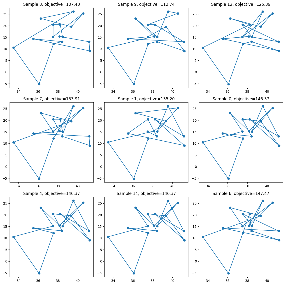
Let’s display the optimized paths for these samples.

fig, axie = plt.subplots(3, 3, figsize=(12, 12))

for i, ax in enumerate(axie.flatten()):
    if i >= len(feasible_ids):
        break
    s = feasible_ids[i]
    x = sample_set.extract_decision_variables("x", s)
    path = sample_to_path(x)
    xs = [ulysses16_points[i][0] for i in path] + [ulysses16_points[path[0]][0]]
    ys = [ulysses16_points[i][1] for i in path] + [ulysses16_points[path[0]][1]]
    ax.plot(xs, ys, marker='o')
    ax.set_title(f"Sample {s}, objective={sample_set.objectives[s]:.2f}")

plt.tight_layout()
plt.show()