Solving Optimization Problems with SCIP

To understand how to use jijmodeling, let’s solve the knapsack problem on this page. However, since jijmodeling is a tool for describing mathematical models, it cannot solve optimization problems on its own. Therefore, we will solve it in combination with the mathematical optimization solver SCIP.

To use jijmodeling with SCIP, you need to install a Python package called ommx-pyscipopt-adapter (GitHub, PyPI). Please install it with the following command:

pip install ommx-pyscipopt-adapter

Problem Setting

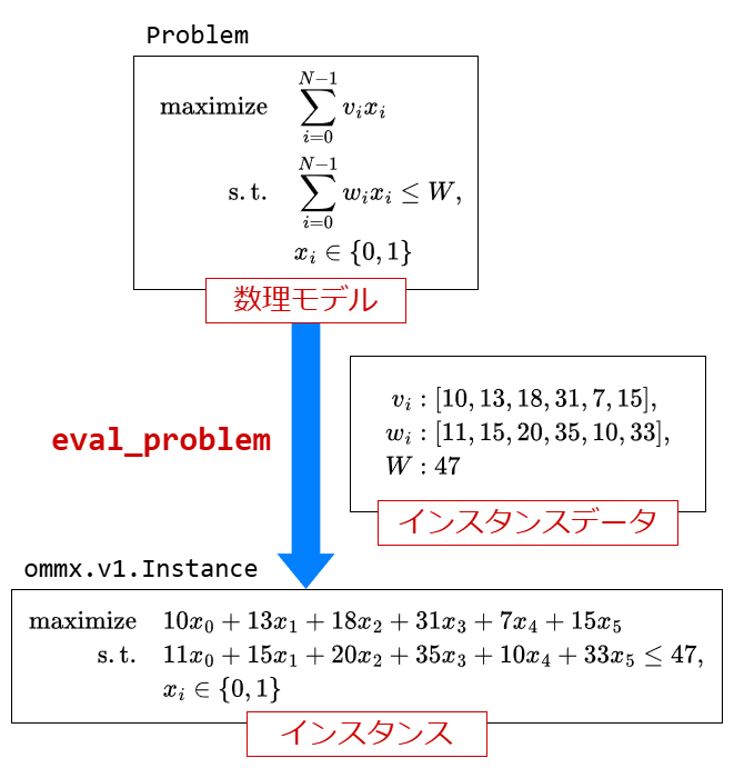
The knapsack problem can be formulated as a mathematical model as follows:

\[\begin{split} \begin{align*} \mathrm{maximize} \quad & \sum_{i=0}^{N-1} v_i x_i \\ \mathrm{s.t.} \quad & \sum_{i=0}^{n-1} w_i x_i \leq W, \\ & x_{i} \in \{ 0, 1\} \end{align*} \end{split}\]

Hint

For more details on the formulation of the knapsack problem, please refer to here.

The meaning of each parameter in this mathematical model is as follows:

Parameter	Description
\(N\)	Total number of items
\(v_{i}\)	Value of item \(i\)
\(w_{i}\)	Weight of item \(i\)
\(W\)	Weight capacity of the knapsack

In this explanation, we will solve an instance obtained by inputting the following values into the parameters \(v_{i}, w_{i}, W\) of the above mathematical model:

Parameter	Value
\(v_{i}\)	[10, 13, 18, 31, 7, 15]
\(w_{i}\)	[11, 15, 20, 35, 10, 33]
\(W\)	47

What is an instance?

In jijmodeling, an instance is a mathematical model with specific values assigned to its parameters.

Procedure for Generating an Instance

Using jijmodeling, you can generate an instance to input into the solver in the following three steps:

1. Formulate the knapsack problem with jijmodeling

2. Register instance data in the Interpreter object

3. Convert the mathematical model to an instance using the Interpreter object

Step1. Formulate the Knapsack Problem with JijModeling

The following Python code formulates the knapsack problem using jijmodeling:

import jijmodeling as jm

# Value of items
v = jm.Placeholder("v", ndim=1)
# Weight of items
w = jm.Placeholder("w", ndim=1)
# Weight capacity of the knapsack
W = jm.Placeholder("W")
# Total number of items
N = v.len_at(0, latex="N")
# Decision variable: 1 if item i is in the knapsack, 0 otherwise
x = jm.BinaryVar("x", shape=(N,)) 
# Index running over the assigned numbers of items
i = jm.Element("i", belong_to=(0, N))

problem = jm.Problem("problem", sense=jm.ProblemSense.MAXIMIZE)
# Objective function
problem += jm.sum(i, v[i] * x[i])
# Constraint: Do not exceed the weight capacity of the knapsack
problem += jm.Constraint("Weight Constraint", jm.sum(i, w[i] * x[i]) <= W)
problem

\[\begin{split}\begin{array}{cccc}\text{Problem:} & \text{problem} & & \\& & \max \quad \displaystyle \sum_{i = 0}^{N - 1} v_{i} \cdot x_{i} & \\\text{{s.t.}} & & & \\ & \text{Weight Constraint} & \displaystyle \sum_{i = 0}^{N - 1} w_{i} \cdot x_{i} \leq W & \\\text{{where}} & & & \\& x & 1\text{-dim binary variable}\\\end{array}\end{split}\]

Hint

For more details on how to formulate with jijmodeling, please refer to here.

Step2. Register Instance Data in the Interpreter Object

Prepare the instance data to be input into the Placeholder of the mathematical model formulated in Step1, and register it in the Interpreter object.

You can register instance data by passing a dictionary with the following keys and values to the constructor of the Interpreter class:

• Key: String set in the name property of the Placeholder object

• Value: Data to be input

instance_data = {
    "v": [10, 13, 18, 31, 7, 15],  # Data of item values
    "w": [11, 15, 20, 35, 10, 33], # Data of item weights
    "W": 47,                       # Data of the knapsack's weight capacity
}
interpreter = jm.Interpreter(instance_data)

Step3. Convert the Mathematical Model to an Instance Using the Interpreter Object

To convert the mathematical model to an instance, use the Interpreter.eval_problem method. By passing the Problem object to the eval_problem method of the Interpreter object with registered instance data, the Placeholder in the Problem object will be filled with the instance data and converted to an instance:

instance = interpreter.eval_problem(problem)

Hint

The return value of Interpreter.eval_problem is an ommx.v1.Instance object. For more details about OMMX, please refer to here.

Solving the Optimization Problem

Now, let’s solve the instance obtained in Step3 with the optimization solver SCIP. The following Python code can be used to obtain the optimal value of the objective function:

from ommx_pyscipopt_adapter import OMMXPySCIPOptAdapter

# Solve through SCIP and retrieve results as an ommx.v1.Solution
solution = OMMXPySCIPOptAdapter.solve(instance)

print(f"Optimal value of the objective function: {solution.objective}")

Optimal value of the objective function: 41.0

In addition, you can display the state of the decision variables as a pandas.DataFrame object using the decision_variables property of solution:

solution.decision_variables[["name", "subscripts", "value"]]

	name	subscripts	value
id
0	x	[0]	1.0
1	x	[1]	1.0
2	x	[2]	1.0
3	x	[3]	0.0
4	x	[4]	0.0
5	x	[5]	0.0

Hint

ommx_pyscipopt_adapter の model_to_solution の返却値は ommx.v1.Solution オブジェクトです。OMMXについて詳しく知りたい場合はこちらを参照してください。