Expressions

What is an Expression?

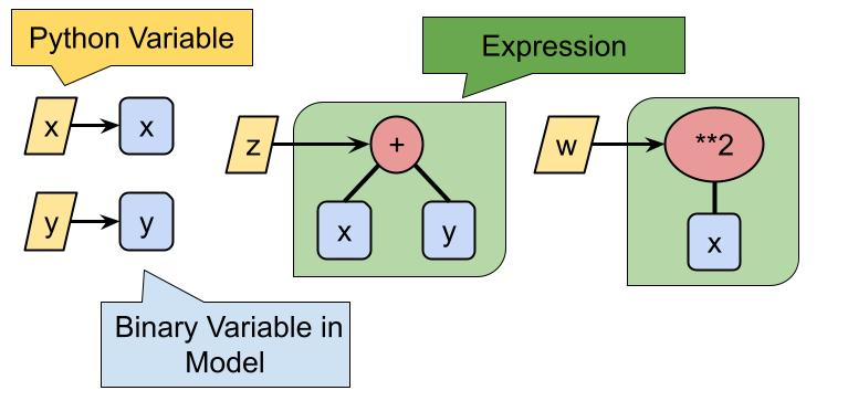
Let’s consider binary operations or unary operations on integer or real variables. For example, \(x+y\) or \(x^2\). Corresponding operations are also possible for variables defined in jijmodeling, and the results are called “expressions”.

import jijmodeling as jm

x = jm.BinaryVar("x")
y = jm.BinaryVar("y")
z = x + y
w = x ** 2

x and y are BinaryVar objects, and z and w are “expressions”. Note that these are “dependent variables” and are different from what we call “decision variables”.

Built-in Operations

Python’s built-in operators (e.g., +) can be used for both decision variables (e.g., BinaryVar) and Placeholder.

x = jm.BinaryVar("x")
y = jm.BinaryVar("y")
z = x + y
repr(z)

"BinaryVar(name='x', shape=[]) + BinaryVar(name='y', shape=[])"

Such operations are algebraic processing (i.e., constructing expression trees). You can check the contents of the expression tree using Python’s built-in repr function. In a Jupyter environment, you can also get a more beautiful display using LaTeX.

Degree of Expressions

Since built-in operations are not limited to linear operations, a function is_linear is provided to determine whether an expression is linear.

x = jm.BinaryVar("x")
jm.is_linear(x)  # True

w = x ** 2
jm.is_linear(w)  # False

Functions such as is_quadratic and is_higher_order are also provided to check the degree of expressions.

Comparison Operations

Equality operator == and other comparison operators (e.g., <=) can also be used to construct equality and inequality constraints. Note that to check if two expression trees are the same, you should use the is_same function instead of the equality operator ==.

x = jm.BinaryVar("x")
y = jm.BinaryVar("y")
repr(x == y)

"BinaryVar(name='x', shape=[]) == BinaryVar(name='y', shape=[])"

jm.is_same(x, y)

False

Indexing and Summation

Similar to Python’s built-in list and numpy.ndarray, jijmodeling supports indexing elements of multi-dimensional decision variables and parameters.

x = jm.BinaryVar("x", shape=(3, 4))
x[0, 2]

\[\displaystyle x_{0, 2}\]

Note

x[0][2] and x[0, 2] refer to the same thing.

x[0, 2] is also an expression. This is similar to the expression tree of x with the unary operator **2 applied. x[0] is the expression tree of x with the unary operator [0] applied to take the 0th element. Also, if the expression does not contain decision variables, it can be specified as an index.

x = jm.BinaryVar("x", shape=(3, 4))
n = jm.Placeholder("n")
x[2*n, 3*n]

\[\displaystyle x_{2 \cdot n, 3 \cdot n}\]

There is a class Element for indexing. This can be used to represent variables \(n\) in summation.

\[ \sum_{n=0}^{N-1} x_n . \]

In jijmodeling, three steps are required to represent summation.

N = jm.Placeholder("N")
x = jm.BinaryVar("x", shape=(N,))

# Step1. Introduce variable $n$ in summation with range [0, N-1]
n = jm.Element('n', belong_to=(0, N))

# Step2. Create expression $x_n$ using index access
xn = x[n]

# Step3. Sum $x_n$ along variable $n$
jm.sum(n, xn)

\[\displaystyle \sum_{n = 0}^{N - 1} x_{n}\]

\[ \mathrm{jm.sum(\overbrace{n}^{subscript}, \underbrace{x[n]}_{operand})} \]

Tip

Simple summations like the above can be written in shorthand.

N = jm.Placeholder('N')
x = jm.BinaryVar(name='x', shape=(N,))
sum_x = x[:].sum()

Since Element objects themselves can be treated as expressions, you can also write \(\sum_n n x_n\) as follows.

jm.sum(n, n * x[n])

\[\displaystyle \sum_{n = 0}^{N - 1} n \cdot x_{n}\]

The result of jm.sum is also an expression. Therefore, you can easily describe models that include the same expression as follows.

n = jm.Element('n', belong_to=(0, N))
sum_x = jm.sum(n, x[n])
sum_x * (1 - sum_x)

\[\displaystyle \sum_{n = 0}^{N - 1} x_{n} \cdot \left(- \sum_{n = 0}^{N - 1} x_{n} + 1\right)\]

Summation over a Set

In mathematical models, summation over a set \(V\) is often performed. For example, the following summation.

\[ \sum_{v \in V} x_v . \]

In this summation, non-continuous indices (e.g., \([1, 4, 5, 9]\) or \([2, 6]\)) are used along the set \(V\).

Tip

Summation over a set is often used in one-hot constraints for a given set \(V\).

\[ \sum_{v \in V} x_v = 1 \]

All expressions explained on this page can also be used as the second argument of the Constraint object.

N = jm.Placeholder('N')
x = jm.BinaryVar('x', shape=(N,))

# Define set $V$ as a Placeholder object
V = jm.Placeholder('V', ndim=1)

# Define variable $v$ moving along $V$
v = jm.Element('v', belong_to=V)

# Sum along $V$
sum_v = jm.sum(v, x[v])

Also, the actual data for the set \(V\) needs to be specified as follows.

import jijmodeling_transpiler as jmt

problem = jm.Problem('Iterating over a Set')
problem += sum_v

instance_data = { "N": 10, "V": [1, 4, 5, 9]}
compiled_model = jmt.core.compile_model(problem, instance_data)

Jagged Arrays

Sometimes, we need to consider groups of sets like \(C_\alpha\). For example, when setting K-hot constraints.

\[ \sum_{i \in C_\alpha} x_i = K_\alpha. \]

These sets \(C_\alpha\) may have different numbers of elements. For example, as follows.

\[\begin{split} \begin{align*} C_1 &= [1, 4, 5, 9], \\ C_2 &= [2, 6], \\ C_3 &= [3, 7, 8] \end{align*} \end{split}\]

You can represent such “jagged” arrays using Placeholder objects.

N = jm.Placeholder('N')
x = jm.BinaryVar('x', shape=(N,))

# Define a 2-dimensional Placeholder object
C = jm.Placeholder('C', ndim=2)

# Define the number of K-hot constraints
# Note that the length in the 0th dimension cannot be obtained because it is a "jagged" array
M = C.len_at(0, latex="M")

K = jm.Placeholder('K', ndim=1)

# Define the index $/alpha$
a = jm.Element(name='a', belong_to=(0, M), latex=r"\alpha")
# Define the variable moving along each $C_/alpha$
i = jm.Element(name='i', belong_to=C[a]) 

# Define the K-hot constraint
k_hot = jm.Constraint('k-hot_constraint', jm.sum(i, x[i]) == K[a], forall=a)

Also, the actual data for \(C\) needs to be passed as follows.

problem = jm.Problem('K-hot')
problem += k_hot

instance_data = {
    "N": 4,
    "C": [[1, 4, 5, 9],
          [2, 6],
          [3, 7, 8]],
    "K": [1, 1, 2],
}
compiled_model = jmt.core.compile_model(problem, instance_data)

Summation over Multiple Indices

Consider a case where multiple summations are included, such as the following.

\[ \sum_{i, j} Q_{ij} x_{ij} \]

Such a case can be implemented in jijmodeling as follows.

# Define variables
Q = jm.Placeholder('Q', ndim=2)
I = Q.shape[0]
J = Q.shape[1]
x = jm.BinaryVar('x', shape=(I, J))
i = jm.Element(name='i', belong_to=(0, I))
j = jm.Element(name='j', belong_to=(0, J))
# Sum along $i$ and $j$
sum_ij = jm.sum([i, j], Q[i, j]*x[i, j])

When there are multiple summations, you can specify the first argument of jm.sum as a list [subscript1, subscript2, ...] instead of using jm.sum multiple times. Of course, this results in the same mathematical model as using jm.sum multiple times because \(\sum_{i, j} = \sum_{i} \sum_{j}\).

sum_ij = jm.sum(i, jm.sum(j, Q[i, j]*x[i, j]))

Conditional Summation

Consider a case where summation is taken over indices that satisfy a specific condition, such as the following.

\[ \sum_{i<U} x_i \]

Such a case can be implemented using jijmodeling as follows.

# Define variables
I = jm.Placeholder('I')
x = jm.BinaryVar('x', shape=(I,))
i = jm.Element(name='i', belong_to=(0, I))
U = jm.Placeholder('U')
# Sum over indices that satisfy $i<U$
sum_i = jm.sum((i, i<U), x[i])

To sum over indices that satisfy a specific condition, you need to specify a tuple (index, condition) as the first argument of jm.sum.

\[ \mathrm{jm.sum((\underbrace{i}_{index}, \overbrace{i<U}^{condition}), \underbrace{x[i]}_{operand})} \]

Comparison operators <, <=, >=, >, ==, != and logical operators &, | and their combinations can be used as conditions. For example,

\[\begin{split} \sum_{\substack{i < U \\ i!=N}} d_i x_i \end{split}\]

can be implemented as follows.

# Define variables
d = jm.Placeholder('d', ndim=1)
I = d.shape[0]
x = jm.BinaryVar('x', shape=(I,))
U = jm.Placeholder('U')
N = jm.Placeholder('N')
i = jm.Element(name='i', belong_to=(0, I))
# Sum over indices that satisfy $i<U$ and $i≠N$
sum_i = jm.sum((i, (i<U)&(i!=N)), d[i]*x[i])

\[ \mathrm{jm.sum((\underbrace{i}_{subscript}, \overbrace{(i<U)}^{condition 1} \underbrace{\&}_{logical operator} \overbrace{(i!=N)}^{condition 2}), \underbrace{d[i]*x[i ]}_{operand})} \]

Conditional Summation with Multiple Conditions

Consider a case where there are conditions on multiple indices in the summation, such as the following.

\[\begin{split} \sum_{\substack{i>L \\ i!=N}} \sum_{j<i} R_{ij} x_{ij} \end{split}\]

Such a case can be implemented in jijmodeling as follows.

# Define variables
R = jm.Placeholder('R', ndim=2)
I = R.shape[0]
J = R.shape[1]
x = jm.BinaryVar('x', shape=(I, J))
i = jm.Element(name='i', belong_to=(0, I))
j = jm.Element(name='j', belong_to=(0, J))
N = jm.Placeholder('N')
L = jm.Placeholder('L')
# Sum over indices that satisfy $i>L$, $i≠N$, and $j<i$
sum_ij = jm.sum([(i, (i>L)&(i!=N)), (j, j<i)], R[i, j]*x[i, j])

You need to specify the first argument of jm.sum as [(index 1, condition of index 1), (index 2, condition of index 2), ...]. By specifying it as [(index1, condition of index1), (index2, condition of index2), ...], you can describe multiple summation operations with conditions on each index.

Caution

[(j, j<i), (i, (i>L)&(i!=N))] will cause an error because \(i\) is not defined at the point of \(j<i\). This corresponds to the fact that you can write \(\sum_{\substack{i>L \\ i!=N}} \left( \sum_{j<i} \cdots \right)\) in an expression, but you cannot write \(\sum_{j<i} \left( \sum_{\substack{i>L \\ i!=N}} \cdots \right)\). Be careful about the order in which you impose conditions on indices in multiple summations.