Formulating Models

What is a model? Why not use solvers directly?

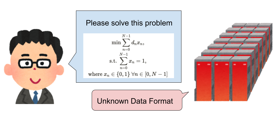
jijmodeling is a modeler library that converts mathematical models readable by humans into data formats readable by computers. There are several types of optimization problems, and solvers specific to those problems only accept solver-specific data formats. Therefore, it is necessary to convert mathematical models into solver-specific data formats. By using jijmodeling, you can describe mathematical models in a single mathematical way and then adapt them to solver- or instance-specific details.

Example of a Mathematical Model

Here we consider a simple binary linear minimization problem with \(N\) real coefficients \(d_n\).

\[\begin{split} \min \sum_{n=0}^{N−1}d_n x_n, \\ \text{s.t.} \space \sum_{n=0}^{N-1} x_n = 1, \\ \text{where} \space x_n \in \{0,1\} \space \forall n \in [0, N-1] \end{split}\]

This problem is a good example to learn the basic usage of jijmodeling. Specifically, you can learn:

• Define decision variables \(x_n\) and placeholders \(N\) and \(d_n\)

• Set the minimization of \(\sum_{n=0}^{N-1} d_n x_n\) as the objective function

• Set the equality constraint \(\sum_{n=0}^{N-1} x_n = 1\)

For more practical and comprehensive examples, please refer to the Learn section of the JijZept documentation site.

Creating a Problem Object

Let’s actually use jijmodeling. First, we need to import it.

import jijmodeling as jm
jm.__version__   # 1.8.0

'1.12.4'

Caution

Before running the following code, it is strongly recommended to ensure that the version of jijmodeling in your environment matches this document.

Now, let’s build a mathematical model using jijmodeling.

# Define the 'parameters'
d = jm.Placeholder("d", ndim=1)
N = d.len_at(0, latex="N")

# Define the 'decision variables'
x = jm.BinaryVar("x", shape=(N,))

# Prepare the index for summation
n = jm.Element('n', belong_to=(0, N))

# Create an object to manage the mathematical model
problem = jm.Problem('my_first_problem')
# Set the objective function
problem += jm.sum(n, d[n] * x[n])
# Set the constraint
problem += jm.Constraint("onehot", jm.sum(n, x[n]) == 1)

# Display the mathematical model
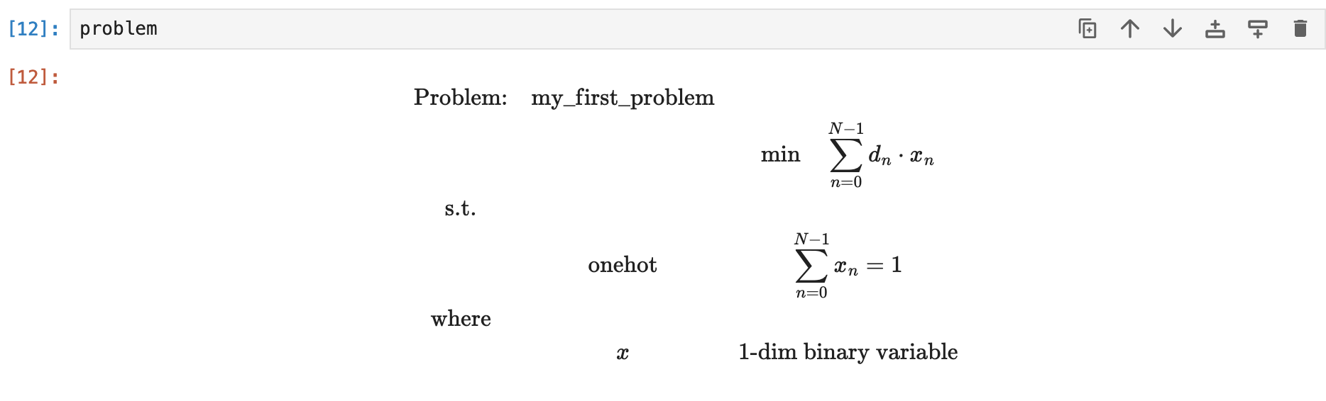
problem

\[\begin{split}\begin{array}{cccc}\text{Problem:} & \text{my\_first\_problem} & & \\& & \min \quad \displaystyle \sum_{n = 0}^{N - 1} d_{n} \cdot x_{n} & \\\text{{s.t.}} & & & \\ & \text{onehot} & \displaystyle \sum_{n = 0}^{N - 1} x_{n} = 1 & \\\text{{where}} & & & \\& x & 1\text{-dim binary variable}\\\end{array}\end{split}\]

Did you understand which part of the code corresponds to the above mathematical model? In this page, we will explain the content and operations of each part of the code in more detail.

Jupyter Environment

In environments like Jupyter Notebook, you can display the contents of the Problem object as shown in the image below. This allows you to interactively debug the model.

Decision Variables and Parameters

The above mathematical model has two types of ‘variables’: ‘decision variables’ and ‘parameters’. In jijmodeling, these are identified by the class used to declare the ‘variables’.

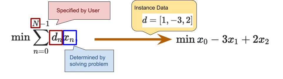
• The value of \(x_n\) is determined by solving the problem, so it is called a ‘decision variable’.

  • In this problem, the binary variable \(x_n \in \{0, 1\}\) is declared with BinaryVar. Other classes that can define decision variables include IntegerVar and ContinuousVar.

  • For more detailed explanations, refer to Types of Decision Variables.

• The values of \(N\) and \(d\) are ‘parameters’ specified by the user.

  • This problem is parameterized by \(N\) and \(d\).

  • The actual values of the ‘parameters’ are not specified within the Problem object.

  • ‘Parameters’ can be considered as containers for the ‘instance data’ of the problem. Specific instances have different values, but jijmodeling can describe mathematical models in a way that does not depend on specific values.

  • Most ‘parameters’ are represented by explicitly defined Placeholder objects like d in the code above.

  • \(N\) is defined as the number of elements of \(d\), and \(N\) is treated as an ‘implicit parameter’. This clarifies the meaning of \(N\) in the mathematical model, and you only need to specify \(d\) to generate an instance.

What is an Object?

In Python, every value has a type. For example, 1 is of type int, and 1.0 is of type float. You can get the type using the built-in function type, like type(1.0). For a type A, a value of type A is called an A object.

Multidimensional Variables

You can define variables that can use indices like arrays or matrices. In the above mathematical model, we want to define \(N\) coefficients \(d_n\) and \(N\) decision variables \(x_n\), so let’s define a 1-dimensional Placeholder object d and a 1-dimensional BinaryVar object x. For Placeholder, it is sufficient to specify that it is 1-dimensional without specifying the number of values. On the other hand, for decision variables, you need to specify the number of dimensions and their length. However, in jijmodeling, you can define the length as a ‘parameter’, so you can write it as follows without using numbers.

# Define the coefficients d
d = jm.Placeholder("d", ndim=1)
# Define N as the length of $d$
N = d.len_at(0, latex="N")
# Define the decision variables $x$ using $N$
x = jm.BinaryVar("x", shape=(N,))

N is of type ArrayLength and represents the number of elements of the Placeholder object d. The 0 given as the first argument of len_at means to count the number of elements in the 0th dimension, which is necessary because Placeholder can have any number of dimensions.

Note

Summation and indices will be explained in more detail on the next page.

Objective Function

Next, let’s set \(\sum_{n=0}^{N-1} d_n x_n\) as the objective function to minimize in the Problem object. However, since \(N\) is not fixed at the stage of constructing the Problem object, we cannot write a Python for loop. So, how should we perform the summation?

To solve this question, jijmodeling has a dedicated sum function.

n = jm.Element('n', belong_to=(0, N))
sum_dx = jm.sum(n, d[n] * x[n])

Element is a new type of variable corresponding to an index within a certain range. Consider the following case:

Given \(n \in [0, N-1]\), take the \(n\)-th element \(d_n\) of \(d \in \mathbb{R}^N\)

In jijmodeling, you can represent \(d_n\) as d[n] using the Element object n corresponding to \(n \in [0, N-1]` and the `Placeholder` object `d` corresponding to \)d\(. Note that the `Element` object has a valid range specified. Then, to represent the summation \)\sum_{n} d_n x_n\(, use the dedicated `sum` function of `jijmodeling`. Specify the `Element` object `n` representing the range to sum over as the first argument, and the expression to sum `d[n] * x[n]` as the second argument. This defines the expression `sum_dx` representing \)\sum_{n} d_n x_n$.

Note

Expressions will be explained in more detail on the next page.

Then, you can create a Problem instance and add sum_dx to set \(\sum_n d_n x_n\) as the objective function as follows.

problem = jm.Problem('my_first_problem')
problem += sum_dx

Problem objects are minimization problems by default. If you want to maximize the objective function, specify the sense argument when constructing the Problem as follows.

problem = jm.Problem('my_first_problem', sense=jm.ProblemSense.MAXIMIZE)

Equality Constraints

Finally, let’s create a Constraint object corresponding to the equality constraint.

\[ \sum_{n=0}^{N-1} x_n = 1 \]

Using the sum function explained above, you can write this constraint as follows.

jm.sum(n, x[n]) == 1

\[\displaystyle \sum_{n = 0}^{N - 1} x_{n} = 1\]

Note that == in jijmodeling expressions returns a new jijmodeling expression, unlike regular Python. Also, Constraint objects require the name of the constraint as the first argument and the comparison expression as the second argument. (In jijmodeling, you can use ==, <=, and >= as comparison expressions) By adding the constructed Constraint object to the Problem object, you can add constraints to the mathematical model.

problem += jm.Constraint("onehot", jm.sum(n, x[n]) == 1)

Note

Constraints and penalties will be explained in more detail on the next page.