Notebook 4: QPE and Resource Estimation

Quantum Phase Estimation (QPE) is an algorithm that estimates the eigenphase $\phi$ associated with an eigenstate $|\psi\rangle$ of a unitary $U$ :

U|\psi\rangle=e^{2\pi i\phi}|\psi\rangle

(1)

In this notebook, we first build the QPE circuit by hand and then compare it with qmc.qpe from the Qamomile stdlib.

1. How QPE works¶

QPE uses two quantum registers with different roles.

The target register holds the eigenstate $|\psi\rangle$ of $U$ .
The counting register consists of $n$ qubits and holds an $n$ -bit approximation of the eigenphase. Its initial state is $|0\rangle^{\otimes n}$ .

The mechanism that transfers the eigenphase from the target to the counting register is phase kickback. Applying a controlled- $U$ with a single control in $|+\rangle$ and the target in $|\psi\rangle$ gives

\frac{|0\rangle|\psi\rangle+|1\rangle U|\psi\rangle}{\sqrt2} = \frac{|0\rangle+e^{2\pi i\phi}|1\rangle}{\sqrt2}|\psi\rangle

(2)

The target returns to the same eigenstate, and only the eigenphase appears as a relative phase on the control. QPE extends this operation to $n$ qubits and reads out the phase in the following three stages.

1. Prepare a uniform superposition¶

Let $N=2^n$ . We prepare $|\psi\rangle$ in the target and apply Hadamards to the counting register. This gives a uniform superposition of the $N$ computational basis states,

|\Psi_1\rangle = \frac{1}{\sqrt N} \sum_{y=0}^{N-1}|y\rangle|\psi\rangle.

(3)

2. Accumulate the phase with controlled powers¶

Write the basis state as $y=\sum_{k=0}^{n-1}y_k2^k$ . We apply $U^{2^k}$ to the target, controlled by the $k$ -th counting qubit. As a result,

|\Psi_2\rangle = \frac{1}{\sqrt N} \sum_{y=0}^{N-1} e^{2\pi i\phi y}|y\rangle|\psi\rangle

(4)

The information about $\phi$ is now recorded in the amplitudes.

3. Decode with the inverse QFT and measure¶

If $\phi=a/N$ can be represented with $n$ bits, the counting register is now in the state $\operatorname{QFT}_N|a\rangle$ . Applying the inverse QFT therefore gives

|\Psi_3\rangle=|a\rangle|\psi\rangle

(5)

Measuring the counting register yields the integer $a$ , and the phase estimate is

\widetilde{\phi}=\frac{a}{2^n}

(6)

If $\phi$ cannot be represented exactly with $n$ bits, the measurement outcomes are distributed around the closest values. Adding one more bit halves the phase resolution $2^{-n}$ , but it also doubles the largest power of the controlled unitary.

The example used in this notebook¶

We take the phase gate with $\theta=3\pi/4$ , $P(\theta)|1\rangle=e^{i\theta}|1\rangle$ , as the unitary whose phase we want to estimate. The phase to be found is then $\phi=\theta/(2\pi)=3/8=0.011_2$ . Since this phase can be represented exactly with 3 qubits, QPE should return the computational basis state $|011\rangle$ .

import math

import matplotlib.pyplot as plt

import qamomile.circuit as qmc
from qamomile.qiskit import QiskitTranspiler

SHOTS = 512
THETA = 3.0 * math.pi / 4.0
EXPECTED_PHASE = 3.0 / 8.0


@qmc.qkernel
def phase_gate(q: qmc.Qubit, theta: qmc.Float) -> qmc.Qubit:
    """Apply the phase $e^{i\\theta}$ to the eigenstate $|1\\rangle$."""
    return qmc.p(q, theta)

2. Build QPE by hand¶

We first defined the unitary that QPE receives as phase_gate. In Qamomile, the unitary passed to QPE is also an ordinary qkernel. The phase gate in this example implements

P(\theta)|0\rangle=|0\rangle,\qquad P(\theta)|1\rangle=e^{i\theta}|1\rangle

(7)

If we prepare the target in $|1\rangle$ , the eigenvalue is $e^{i\theta}=e^{2\pi i\phi}$ , so the phase returned by QPE is $\phi=\theta/(2\pi)$ .

In manual_qpe below, the QPE steps we saw above are mapped directly onto code.

Allocate the counting register with qubit_array(n) and the target register with qubit()
Prepare the target register in the eigenstate $|1\rangle$ with x(target), and put the counting register into a superposition with h(counting)
Use control(phase_gate) to apply the unitary from each counting qubit with power=2**k
Decode the phase with iqft(counting), cast it to QFixed, and then measure it

QFixed is the Qamomile type for treating a quantum register as a fixed-point number. With int_bits=0, all $n$ qubits are interpreted as the fractional part, so the integer $a$ after the inverse QFT is read out as the phase $a/2^n$ .

@qmc.qkernel
def manual_qpe(
    n: qmc.UInt,
    theta: qmc.Float,
) -> qmc.Float:
    """Build QPE from Hadamards, controlled powers, and an inverse QFT."""
    counting = qmc.qubit_array(n, "counting")
    target = qmc.qubit("target")

    target = qmc.x(target)
    counting = qmc.h(counting)

    controlled_phase = qmc.control(phase_gate)
    for k in qmc.range(n):
        counting[k], target = controlled_phase(
            counting[k],
            target,
            theta=theta,
            power=2**k,
        )

    counting = qmc.iqft(counting)
    phase = qmc.cast(counting, qmc.QFixed, int_bits=0)
    return qmc.measure(phase)


manual_qpe.draw(n=3, theta=THETA, fold_loops=False)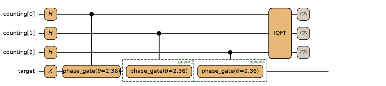

qmc.control(phase_gate) creates a controlled unitary from an existing qkernel. This means there is no need to rewrite the unitary itself for QPE.

power=2**k realizes the operation “controlled- $U^{2^k}$ ”.

The final qmc.iqft(counting) converts the phase pattern back into the integer $a$ . The following qmc.cast(counting, qmc.QFixed, int_bits=0) interprets the same quantum register as the fixed-point number $a/2^n$ . For example, for $|011\rangle$ ,

\frac{1\cdot2^0+1\cdot2^1+0\cdot2^2}{2^3} =\frac38

(8)

cast is not an operation that adds quantum gates. As a result, it returns the type Float value.

transpiler = QiskitTranspiler()
manual_executable = transpiler.transpile(
    manual_qpe,
    bindings={"n": 3, "theta": THETA},
)
manual_result = manual_executable.sample(
    transpiler.executor(),
    shots=SHOTS,
).result()
print("Manual QPE:", manual_result.results)

assert len(manual_result.results) == 1
manual_phase, manual_count = manual_result.results[0]
assert manual_count == SHOTS
assert math.isclose(manual_phase, EXPECTED_PHASE, abs_tol=1e-12)

Manual QPE: [(0.375, 512)]

Because $\phi=3/8$ can be represented exactly with 3 bits, every shot gives the same phase value on a noiseless simulator. For a general phase, several nearby values appear, so sample_result.results must be read as a distribution of measured values and their counts.

3. The built-in `qmc.qpe`¶

Qamomile provides the same procedure as qmc.qpe. Building QPE by hand is well suited to learning and understanding the circuit structure. When assembling more complex algorithms, however, using the algorithms included in the stdlib makes even complex algorithms easy to implement.

The first three arguments of qmc.qpe are:

target: the target qubit or target register prepared in an eigenstate
counting: the counting register in the initial state $|0\rangle^{\otimes n}$
phase_gate: the unitary qkernel whose phase is to be estimated

The remaining keyword arguments are forwarded to the unitary. Here, theta=theta becomes the parameter of phase_gate.

In the hand-built version we wrote qmc.cast(..., qmc.QFixed, int_bits=0) explicitly, but qmc.qpe already includes the same conversion. Therefore, in both implementations, the return value of measure(phase) is not a bit tuple but a Float that has already been decoded to $a/2^n$ .

@qmc.qkernel
def builtin_qpe(
    n: qmc.UInt,
    theta: qmc.Float,
) -> qmc.Float:
    """Measure the phase as a fixed-point number with the Qamomile stdlib QPE."""
    counting = qmc.qubit_array(n, "counting")
    target = qmc.qubit("target")
    target = qmc.x(target)

    phase = qmc.qpe(target, counting, phase_gate, theta=theta)
    return qmc.measure(phase)


builtin_qpe.draw(n=3, theta=THETA, fold_loops=False)

builtin_executable = transpiler.transpile(
    builtin_qpe,
    bindings={"n": 3, "theta": THETA},
)
builtin_result = builtin_executable.sample(
    transpiler.executor(),
    shots=SHOTS,
).result()
print("Built-in QPE:", builtin_result.results)

assert len(builtin_result.results) == 1
builtin_phase, builtin_count = builtin_result.results[0]
assert math.isclose(builtin_phase, EXPECTED_PHASE, abs_tol=1e-12)
assert builtin_count == SHOTS

Built-in QPE: [(0.375, 512)]

@qmc.qkernel
def builtin_qpe(
    n: qmc.UInt, theta: qmc.Float
) -> qmc.Float:
    counting = qmc.qubit_array(n, "counting")
    target = qmc.qubit("target")
    target = qmc.x(target)
 
    phase = qmc.qpe(
        target, counting,
        phase_gate, theta=theta,
    )
    return qmc.measure(phase)

4. Count logical resources from a concrete circuit¶

estimate_resources() does not execute a qkernal. It counts the number of logical qubits and logical gates from the Qamomile IR. We first compare the hand-built and built-in versions on the same 3-bit problem. If the values of the hand-built and stdlib versions agree, we can confirm that the shorter notation is estimated to have the same logical resource breakdown. Note, however, that having the same resource breakdown does not mean that the transpiled circuits are completely identical.

manual_resources = manual_qpe.estimate_resources(inputs={"n": 3, "theta": THETA})
builtin_resources = builtin_qpe.estimate_resources(inputs={"n": 3, "theta": THETA})

for name, resources in [
    ("manual", manual_resources),
    ("built-in", builtin_resources),
]:
    print(
        f"{name:8s}: qubits={resources.qubits}, "
        f"gates={resources.gates.total}, "
        f"two-qubit={resources.gates.two_qubit}"
    )

assert manual_resources.qubits == builtin_resources.qubits == 4
assert manual_resources.gates == builtin_resources.gates

manual  : qubits=4, gates=18, two-qubit=11
built-in: qubits=4, gates=18, two-qubit=11

5. Plug a variable-width Oracle into the built-in QPE¶

So far we have executed a concrete phase gate and counted resources from its circuit. Sometimes, however, you want to study the scaling of the whole QPE before a subroutine such as Hamiltonian simulation has been implemented. qmc.Oracle is an abstract callable object that represents such an unimplemented unitary by its name and signature alone.

In this section, we clearly separate the roles of the symbols.

$n$ : the number of qubits in the target register on which the unitary $U$ acts
$m$ : the number of qubits in the counting register, which estimates the phase with $m$ bits

oracle = qmc.Oracle(
    name="u",
    signature=qmc.CallableSignature(
        inputs=[qmc.Vector[qmc.Qubit]],
        outputs=[qmc.Vector[qmc.Qubit]],
    ),
)

In CallableSignature, we specify Vector[Qubit] → Vector[Qubit] rather than a fixed number of qubits. This lets us reuse the same Oracle for different numbers of qubits $n$ .

Because the unitary passed to the built-in qmc.qpe must be a qkernel, we wrap the Oracle in u_for_qpe, which contains only the Oracle call.

@qmc.qkernel
def u_for_qpe(
    target: qmc.Vector[qmc.Qubit],
) -> qmc.Vector[qmc.Qubit]:
    """Unitary qkernel that passes a variable-width Oracle to the built-in QPE."""
    return oracle(target)


@qmc.qkernel
def qpe_model(
    n: qmc.UInt,
    m: qmc.UInt,
) -> qmc.QFixed:
    """Build a symbolic resource model of QPE with a variable-width Oracle."""
    target = qmc.qubit_array(n, name="target")
    counting = qmc.qubit_array(m, name="counting")

    # In an actual QPE, the target would be prepared in an eigenstate of U here.
    return qmc.qpe(target, counting, u_for_qpe)

Because we give no concrete inputs to estimate_resources(), the result is an algebraic expression in $n$ and $m$ . In this example, the number of qubits is $m+n$ .

In addition, since qmc.qpe calls controlled- $U^{2^k}$ for counting qubit $k$ , in a model that counts $U^{2^k}$ as $2^k$ queries to the base Oracle $U$ , the number of queries is

1+2+\cdots+2^{m-1}=2^m-1

(9)

With UnknownResourcePolicy.OPAQUE_CALL, Qamomile does not raise an error for an Oracle without an implementation. Instead, it records the calls and queries by name.

We do not print gates.total here, so that it is not mistaken for the gate count of the whole algorithm: it contains only the cost of the Hadamards and the inverse QFT in QPE, and not the cost of the Oracle. Also, because this model has no Oracle body, it cannot be transpiled and executed.

symbolic_resources = qpe_model.estimate_resources(
    unknown_policy=qmc.UnknownResourcePolicy.OPAQUE_CALL,
).simplify()

print("Symbolic qubits:", symbolic_resources.qubits)
print("Symbolic Oracle queries:", symbolic_resources.calls.oracle_queries)

Symbolic qubits: m + n
Symbolic Oracle queries: {'u': 2**m - 1}

We can see that the resource estimate is indeed what we expected.

Finally, we can also substitute values into this algebraic estimate to obtain concrete numbers. This is a substitution into a formula, not a circuit construction, so it can be computed quickly.

for n_value, m_value in [(2, 3), (4, 3), (4, 5)]:
    concrete = symbolic_resources.substitute(n=n_value, m=m_value)
    queries = int(concrete.calls.oracle_queries["u"])
    print(f"n={n_value}, m={m_value}: qubits={int(concrete.qubits)}, queries={queries}")
    assert int(concrete.qubits) == n_value + m_value
    assert queries == 2**m_value - 1

n=2, m=3: qubits=5, queries=7
n=4, m=3: qubits=7, queries=7
n=4, m=5: qubits=9, queries=31

Exercise: A phase that cannot be represented with 3 bits¶

Change THETA to 2*pi/3, that is, to $\phi=1/3$ . Because this phase cannot be represented exactly with 3 bits, several measurement outcomes appear. Increasing the number of counting bits makes the phase resolution $2^{-n}$ finer, so confirm that the peak of the distribution approaches $1/3$ .

Specifically, investigate the following two points.

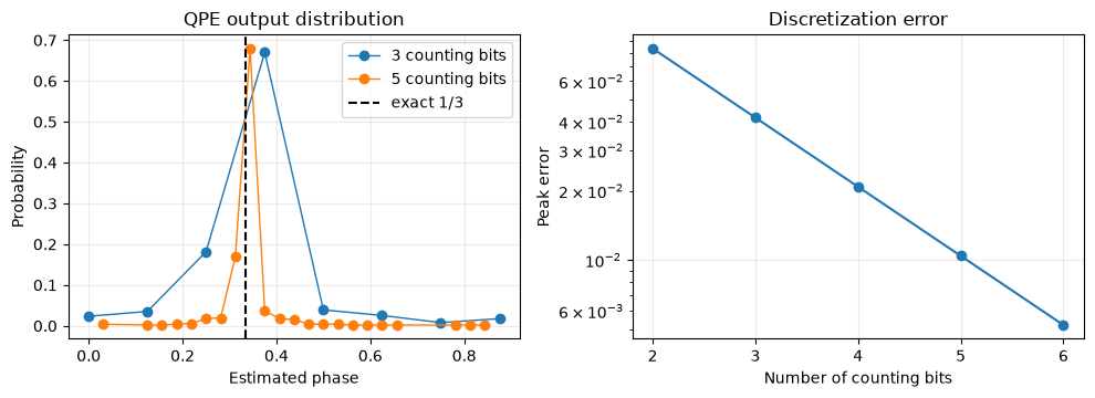
Compare the phase distributions for 3 and 5 counting bits
Increase the number of counting bits from 2 to 6 and confirm that the error between the most frequent value and $1/3$ decreases

# TODO: For theta=2*pi/3, examine the phase distribution and the error versus the number of counting bits.

Example Solution¶

exercise_phase = 1.0 / 3.0
exercise_theta = 2.0 * math.pi * exercise_phase
counting_widths = [2, 3, 4, 5, 6]
phase_distributions = {}
peak_errors = {}

for counting_bits in counting_widths:
    exercise_executable = transpiler.transpile(
        builtin_qpe,
        bindings={"n": counting_bits, "theta": exercise_theta},
    )
    exercise_result = exercise_executable.sample(
        transpiler.executor(),
        shots=SHOTS,
    ).result()
    phase_distributions[counting_bits] = sorted(exercise_result.results)

    peak_phase, _ = max(exercise_result.results, key=lambda item: item[1])
    peak_errors[counting_bits] = abs(peak_phase - exercise_phase)
    print(
        f"counting bits={counting_bits}: "
        f"peak={peak_phase:.5f}, error={peak_errors[counting_bits]:.5f}"
    )

assert all(
    peak_errors[right] < peak_errors[left]
    for left, right in zip(counting_widths, counting_widths[1:], strict=False)
)

fig, axes = plt.subplots(1, 2, figsize=(10, 3.7))

for counting_bits in [3, 5]:
    distribution = phase_distributions[counting_bits]
    phases = [phase for phase, _ in distribution]
    probabilities = [count / SHOTS for _, count in distribution]
    axes[0].plot(
        phases,
        probabilities,
        marker="o",
        linewidth=1,
        label=f"{counting_bits} counting bits",
    )

axes[0].axvline(exercise_phase, color="black", linestyle="--", label="exact 1/3")
axes[0].set(
    xlabel="Estimated phase",
    ylabel="Probability",
    title="QPE output distribution",
)
axes[0].legend()
axes[0].grid(alpha=0.25)

axes[1].plot(
    counting_widths,
    [peak_errors[width] for width in counting_widths],
    marker="o",
)
axes[1].set(
    xlabel="Number of counting bits",
    ylabel="Peak error",
    title="Discretization error",
    yscale="log",
)
axes[1].set_xticks(counting_widths)
axes[1].grid(alpha=0.25)

plt.tight_layout()
plt.show()

counting bits=2: peak=0.25000, error=0.08333
counting bits=3: peak=0.37500, error=0.04167
counting bits=4: peak=0.31250, error=0.02083
counting bits=5: peak=0.34375, error=0.01042
counting bits=6: peak=0.32812, error=0.00521

Summary¶

In QPE, the target is prepared in an eigenstate (or a state with a large overlap with an eigenstate), and Hadamards, controlled- $U^{2^k}$ , and the inverse QFT are applied in turn to the counting register.
The Qamomile stdlib provides several algorithms, including QPE.
The same qkernel can be used both to build an executable circuit and to estimate resources.
Unimplemented subroutines can also be represented as an Oracle, and the number of Oracle queries can be estimated symbolically without assuming an implementation.