Notebook 5: Quantum Optimization with Graph Coloring - Qamomile Tutorial at IEEE Quantum Week 2026

In this notebook, we formulate a graph coloring problem, solve it with QAOA, OpenJij SA, and SCIP, and compare the solutions and execution times.

We work through five steps using a small graph, introducing terms and equations alongside the code.

Step	What we do in this notebook	Main code
1. Formulate	Define variables, an objective function, and constraints	JijModeling’s `problem`
2. Instantiate	Supply the graph and number of colors	`problem.eval()`
3. Conversion	Convert the problem into a QAOA circuit	`QAOAConverter`
4. Solve	Compute expectation values and adjust parameters	`estimate()`, `minimize()`
5. Decode	Recover color assignments from measurement results	`converter.decode()`

We then compare QAOA with classical solvers and benchmark them as the number of vertices increases. QAOA expectation values and final measurements are simulated on a classical computer.

import time

import jijmodeling as jm
import matplotlib.pyplot as plt
import networkx as nx
import numpy as np
import pandas as pd
from ommx_openjij_adapter import OMMXOpenJijSAAdapter
from ommx_pyscipopt_adapter import OMMXPySCIPOptAdapter
from scipy.optimize import minimize

from qamomile.optimization.qaoa import QAOAConverter
from qamomile.qiskit import QiskitTranspiler

NUM_COLORS = 3
FINAL_SHOTS = 2048  # Shots for obtaining color assignments
MAX_EVALS = 100  # Maximum function evaluations for parameter tuning
SA_READS = 500  # Number of SA reads

1. Formulate the Problem¶

In graph coloring, we assign different colors to adjacent vertices: vertices connected by an edge. Here, we fix the number of available colors at three and minimize the number of conflicts, meaning edges whose endpoints have the same color. A value of zero means that the graph has been properly colored with three colors.

We use a four-vertex graph consisting of a triangle with one additional vertex attached. Vertices 0, 1, and 2 each need a different color. Vertex 3 only needs to differ from vertex 2, so it can use the same color as vertex 0 or 1.

graph = nx.Graph([(0, 1), (1, 2), (0, 2), (2, 3)])
positions = nx.spring_layout(graph, seed=7)

plt.figure(figsize=(4.5, 3))
nx.draw(
    graph, pos=positions, with_labels=True,
    node_color="lightgray", node_size=850, width=2,
)
plt.title("Which color should each vertex use?")
plt.show()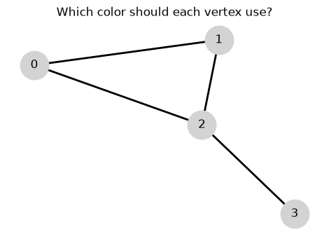

Let $N$ be the number of vertices, $K$ the number of colors, and $E$ the set of edges. The decision variable $x_{v,c}$ is a binary variable: it is 1 when vertex $v$ is assigned color $c$ , and 0 otherwise.

The following formulation minimizes the objective function $f(x)$ , which counts conflicts, subject to the constraint that each vertex is assigned exactly one color.

\begin{aligned} \underset{x\in\{0,1\}^{N\times K}}{\operatorname{minimize}} \quad & f(x)=\sum_{(u,v)\in E}\sum_{c=0}^{K-1}x_{u,c}x_{v,c}\\ \text{subject to}\quad & \sum_{c=0}^{K-1}x_{v,c}=1 \quad(v=0,\ldots,N-1). \end{aligned}

(1)

This is a one-hot constraint: exactly one variable for each vertex must be 1. For example, $x_{v,1} = 1$ means that vertex $v$ is assigned color 1. When this constraint holds, the term $\sum_c x_{u,c}x_{v,c}$ for an edge is 1 if its endpoints have the same color, and 0 otherwise.

An assignment that satisfies the constraints is a feasible solution. The value of the objective function is the objective value. A feasible solution with the smallest objective value is an optimal solution, and that value is the optimal value. In this model, an assignment is feasible as long as each vertex has exactly one color, even if conflicts remain. A feasible solution with objective value 0 is a proper coloring: every edge has endpoints of different colors.

Express the Formulation in JijModeling¶

N, K, and E are placeholders for data that we supply later. x is an array of binary variables with shape (N, K), one for each vertex-color pair.

In the objective, the inner sum() sums over colors, and the outer sum() sums over edges. Constraint(..., domain=N) adds a one-hot constraint for each vertex.

problem = jm.Problem("Graph Coloring")


@problem.update
def _(problem: jm.DecoratedProblem):
    N = problem.Dim()
    K = problem.Dim()
    E = problem.Natural(ndim=2)
    x = problem.BinaryVar(shape=(N, K))
    # Objective: count edges whose endpoints have the same color
    problem += E.rows().map(
        lambda edge: (x[edge[0], :] * x[edge[1], :]).sum()
    ).sum()
    # Constraint: assign exactly one color to each vertex
    problem += problem.Constraint(
        "one-color", lambda v: x[v, :].sum() == 1, domain=N
    )


problem

2. Instantiate the Model¶

An instance is a mathematical model with specific input data supplied. problem.eval(instance_data) substitutes the vertex count, color count, and edges, producing an Instance in the common OMMX data format. The color assignment $x$ has not yet been determined.

Software that solves optimization problems is called a solver. We use this instance to solve the same problem with QAOA, OpenJij SA, and SCIP. Check that the output shows 4 vertices, 3 colors, 12 binary variables, and 4 one-hot constraints.

instance_data = {
    "N": graph.number_of_nodes(),
    "K": NUM_COLORS,
    "E": [list(edge) for edge in graph.edges()],
}
instance = problem.eval(instance_data)
print("vertices:", instance_data["N"])
print("colors:", NUM_COLORS)
print("binary variables:", len(instance.decision_variables))
print("one-hot constraints:", len(instance.constraints))

vertices: 4
colors: 3
binary variables: 12
one-hot constraints: 4

3. Convert the Problem into a QAOA Circuit¶

QUBO (quadratic unconstrained binary optimization) minimizes a quadratic expression in binary variables without explicit constraints. QAOAConverter adds penalties for constraint violations to the original objective, converts the problem into a QUBO, and then converts it into an Ising model. Our QUBO is

F(x)=f(x)+A\sum_{v=0}^{N-1}\left(\sum_{c=0}^{K-1}x_{v,c}-1\right)^2.

(2)

The added term is zero when the one-hot constraints hold and positive when they are violated. For example, setting every variable to zero gives $f(x)=0$ , but incurs a penalty because no colors are assigned. We set $A=|E|+1=5$ . A feasible solution has $F(x)=f(x)\leq |E|$ ; a candidate that violates a constraint has $F(x)\geq A$ . The optimal solution of the QUBO therefore also satisfies the constraints.

Substituting $x=(1-z)/2$ replaces binary variables with spin variables $z\in\{+1,-1\}$ , giving an Ising model. Using the corresponding cost Hamiltonian, transpile(..., p=1) creates a single-layer QAOA circuit. This model needs no auxiliary variables, so the qubit count equals the number of binary variables: $NK=12$ .

normalize_by_abs_max() normalizes the coefficients by dividing them all by the same positive constant. This leaves the bit strings with minimum energy unchanged. Calling executor() without arguments sets up execution using the default simulator.

penalty_weight = graph.number_of_edges() + 1
converter = QAOAConverter(instance, uniform_penalty_weight=penalty_weight)
converter.spin_model.normalize_by_abs_max(replace=True)

transpiler = QiskitTranspiler()
qaoa = converter.transpile(transpiler, p=1)
executor = transpiler.executor()

print("penalty weight:", penalty_weight)
print("QAOA qubits:", converter.spin_model.num_bits)

penalty weight: 5
QAOA qubits: 12

4. Adjust the Circuit Parameters¶

We adjust the QAOA circuit parameters to lower the expected energy, including penalties. With one layer, there are two parameters to adjust: $\gamma,\beta$ .

remove_final_measurements() creates a circuit without measurements for expectation evaluation. energy() uses params[0] as $\gamma$ and params[1] as $\beta$ , then calls executor.estimate() to compute the expectation value. It calculates this directly from the statevector, so no shots are needed here.

We adjust the parameters with minimize(), then obtain color assignments from the final measurements in the next section.

state_circuit = qaoa.quantum_circuit.remove_final_measurements(inplace=False)
hamiltonian = converter.get_cost_hamiltonian()


def energy(params):
    circuit = state_circuit.assign_parameters({
        "gammas[0]": params[0], "betas[0]": params[1],
    })
    return executor.estimate(circuit, hamiltonian)


initial_params = np.random.default_rng(7).uniform(0.0, np.pi, 2)
optimized = minimize(
    energy, initial_params, method="COBYLA",
    options={"maxiter": MAX_EVALS},
)
print("optimized parameters:", optimized.x)

optimized parameters: [3.82315881 2.00087508]

5. Decode Measurements into Color Assignments¶

Using the optimized parameters, we take FINAL_SHOTS measurement shots and call converter.decode() to map each candidate back to the variables of the original OMMX instance. We then evaluate whether it satisfies the one-hot constraints and compute the original objective value $f(x)$ . Measurement results vary from run to run.

The expected energy minimized in the previous section includes penalties. To compare solutions, we use the original objective value without penalties. For a feasible solution, this is the number of conflicts.

best_feasible_or_none() selects the feasible solution with the smallest objective value among those obtained. QAOA does not guarantee that any of its samples satisfy the constraints, so the function returns None if no feasible solution is found.

def best_feasible_or_none(samples):
    if not samples.summary["feasible"].any():
        return None
    return samples.best_feasible


final_sample = qaoa.sample(
    executor,
    shots=FINAL_SHOTS,
    bindings={
        "gammas": [optimized.x[0]],
        "betas": [optimized.x[1]],
    },
).result()
qaoa_samples = converter.decode(final_sample)
qaoa_solution = best_feasible_or_none(qaoa_samples)

if qaoa_solution is None:
    print("No one-hot-feasible sample. Try more shots or another seed.")
else:
    print("best conflicts:", qaoa_solution.objective)
    print("proper coloring:", np.isclose(qaoa_solution.objective, 0))

best conflicts: 0.0
proper coloring: True

Inspect the Color Assignment¶

extract_decision_variables("x") retrieves each (vertex index, color index) pair and its variable value. Because the selected solution satisfies the one-hot constraints, the variables with value 1 identify each vertex’s color.

In the figure, v: c means “vertex index: color index.” Conflicting edges are drawn in red, and their count appears as conflict(s) in the title.

if qaoa_solution is not None:
    values = qaoa_solution.extract_decision_variables("x")
    assignment = {v: c for (v, c), value in values.items() if value > 0.5}
    conflicts = [
        (u, v) for u, v in graph.edges if assignment[u] == assignment[v]
    ]
    palette = plt.get_cmap("tab10")
    plt.figure(figsize=(4.5, 3))
    nx.draw(
        graph, pos=positions,
        labels={v: f"{v}: {assignment[v]}" for v in graph.nodes},
        node_color=[palette(assignment[v]) for v in graph.nodes],
        edge_color=["tab:red" if e in conflicts else "lightgray" for e in graph.edges],
        width=2.5, node_size=1100, font_color="white",
    )
    plt.title(f"QAOA: {len(conflicts)} conflict(s)")
    plt.show()
    print("vertex -> color:", assignment)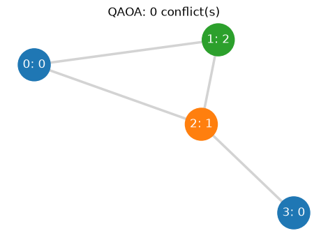

vertex -> color: {0: 0, 1: 2, 2: 1, 3: 0}

6. Compare with Classical Solvers¶

We pass the same instance to OMMX Adapters, which convert it into the format each solver requires. The following two solvers solve the same problem as QAOA.

OpenJij SA runs simulated annealing. We use the same penalty weight as QAOA and set the number of reads to SA_READS.
SCIP handles the original objective and constraints. We use its optimal value as the reference.

For QAOA and SA, we select the feasible solution with the smallest objective value among those obtained. We compare that value with SCIP’s optimal value to check whether the selected solution is optimal.

openjij_samples = OMMXOpenJijSAAdapter.sample(
    instance,
    num_reads=SA_READS,
    uniform_penalty_weight=penalty_weight,
)
openjij_solution = best_feasible_or_none(openjij_samples)

scip_solution = OMMXPySCIPOptAdapter.solve(instance)

We compare the results using the objective value of the original problem.

Column	Meaning
`best`	The smallest objective value among the feasible solutions obtained
`gap`	`best` minus SCIP’s optimal value
`feasible_rate`	Fraction of returned candidates that are feasible (0–1)

best=0 means there are no conflicts; gap=0 means the solution is optimal. For example, if a problem has optimal value 1 and we obtain a feasible solution with objective value 1, then best=1 and gap=0. If no feasible solution is found, best and gap are NaN (missing data). SCIP returns a feasible solution, so we set its feasible_rate to 1.0 here.

solutions = {"QAOA": qaoa_solution, "OpenJij SA": openjij_solution, "SCIP": scip_solution}
comparison = pd.DataFrame([
    {"method": method, "best": np.nan if solution is None else solution.objective}
    for method, solution in solutions.items()
])
comparison["gap"] = comparison["best"] - scip_solution.objective
comparison["feasible_rate"] = [
    qaoa_samples.summary["feasible"].mean(),
    openjij_samples.summary["feasible"].mean(),
    1.0,
]
comparison

7. Benchmark Across Problem Sizes¶

Finally, we vary the number of vertices across 3, 4, 5, and 6, comparing the gap to the optimal value and execution time. We keep the color count fixed at NUM_COLORS. With three colors, these problems use 9, 12, 15, and 18 qubits, respectively.

For each size, we generate a random graph by connecting each pair of vertices with probability 0.5, then add the edges (0, 1), (1, 2), ... to make the graph connected. We fix the random seed for graph generation and pass the same OMMX instance to all three methods. A proper coloring may not exist with the available colors, so we use SCIP to determine the optimal value for each size.

QAOA and SA both use the penalty weight $A=|E|+1$ . QAOA uses one layer. Its final measurement shot count and evaluation budget, and the SA read count, use the shared constants defined at the start.

problem_sizes = [3, 4, 5, 6]

We collect the QAOA steps from Sections 3–5 into solve_with_qaoa(). It returns the selected solution (or None if none is feasible) and the fraction of feasible samples.

The following loop records the time before and after each solver’s processing to calculate elapsed time.

def solve_with_qaoa(instance, penalty_weight, seed):
    converter = QAOAConverter(instance, uniform_penalty_weight=penalty_weight)
    converter.spin_model.normalize_by_abs_max(replace=True)
    transpiler = QiskitTranspiler()
    qaoa = converter.transpile(transpiler, p=1)
    executor = transpiler.executor()

    state_circuit = qaoa.quantum_circuit.remove_final_measurements(inplace=False)
    hamiltonian = converter.get_cost_hamiltonian()

    def energy(params):
        circuit = state_circuit.assign_parameters({
            "gammas[0]": params[0], "betas[0]": params[1],
        })
        return executor.estimate(circuit, hamiltonian)

    initial = np.random.default_rng(seed).uniform(0.0, np.pi, 2)
    optimized = minimize(
        energy, initial, method="COBYLA",
        options={"maxiter": MAX_EVALS},
    )
    sample = qaoa.sample(
        executor,
        shots=FINAL_SHOTS,
        bindings={
            "gammas": [optimized.x[0]],
            "betas": [optimized.x[1]],
        },
    ).result()
    samples = converter.decode(sample)
    return best_feasible_or_none(samples), samples.summary["feasible"].mean()

benchmark_rows = []
for num_vertices in problem_sizes:
    benchmark_graph = nx.gnp_random_graph(
        num_vertices, p=0.5, seed=1000 + num_vertices
    )
    benchmark_graph.add_edges_from((v, v + 1) for v in range(num_vertices - 1))
    benchmark_instance = problem.eval({
        "N": num_vertices,
        "K": NUM_COLORS,
        "E": [list(edge) for edge in benchmark_graph.edges()],
    })
    penalty = benchmark_graph.number_of_edges() + 1
    qubits = num_vertices * NUM_COLORS
    print(f"Solving N={num_vertices}, edges={benchmark_graph.number_of_edges()}, qubits={qubits}")

    started = time.perf_counter()
    scip_best = OMMXPySCIPOptAdapter.solve(benchmark_instance)
    scip_elapsed = time.perf_counter() - started
    reference = scip_best.objective

    started = time.perf_counter()
    sa_samples = OMMXOpenJijSAAdapter.sample(
        benchmark_instance,
        num_reads=SA_READS,
        uniform_penalty_weight=penalty,
    )
    sa_best = best_feasible_or_none(sa_samples)
    sa_rate = sa_samples.summary["feasible"].mean()
    sa_elapsed = time.perf_counter() - started

    started = time.perf_counter()
    qaoa_best, qaoa_rate = solve_with_qaoa(
        benchmark_instance, penalty, seed=7 + num_vertices
    )
    qaoa_elapsed = time.perf_counter() - started
    for method, solution, elapsed, feasible_rate in [
        ("QAOA", qaoa_best, qaoa_elapsed, qaoa_rate),
        ("OpenJij SA", sa_best, sa_elapsed, sa_rate),
        ("SCIP", scip_best, scip_elapsed, 1.0),
    ]:
        best = np.nan if solution is None else solution.objective
        benchmark_rows.append({
            "vertices": num_vertices,
            "qubits": qubits,
            "edges": benchmark_graph.number_of_edges(),
            "method": method,
            "best": best,
            "gap": best - reference,
            "feasible_rate": feasible_rate,
            "seconds": elapsed,
        })

Solving N=3, edges=3, qubits=9
Solving N=4, edges=3, qubits=12
Solving N=5, edges=6, qubits=15
Solving N=6, edges=12, qubits=18

best, gap, and feasible_rate are the same metrics as in Section 6. The following columns also show problem size and execution time.

Column	Meaning
`vertices`	Number of vertices
`qubits`	Number of QAOA qubits
`edges`	Number of edges
`seconds`	Elapsed time in seconds, from problem conversion through solving, solution evaluation, and selection

Timing excludes OMMX instance creation and plotting. If no feasible solution is found, best and gap are NaN, and the next plot omits the gap point for that size.

benchmark = pd.DataFrame(benchmark_rows)
benchmark

fig, axes = plt.subplots(1, 2, figsize=(9, 3.5))
for method, rows in benchmark.groupby("method", sort=False):
    axes[0].plot(rows["vertices"], rows["gap"], "o-", label=method)
    axes[1].plot(rows["vertices"], rows["seconds"], "o-", label=method)

axes[0].set(title="Best feasible solution", ylabel="Gap to SCIP optimum")
axes[1].set(title="End-to-end time", ylabel="Wall-clock time [s]", yscale="log")
for axis in axes:
    axis.set_xlabel("Number of vertices")
    axis.set_xticks(problem_sizes)
    axis.grid(alpha=0.25)
    axis.legend()
fig.suptitle(f"Graph coloring: {NUM_COLORS} colors, QAOA p=1")
plt.tight_layout()
plt.show()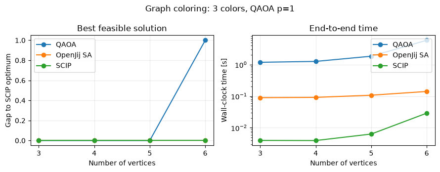

The left plot compares the gap to the optimal value; the right plot compares execution time on a logarithmic vertical scale. For sizes where all methods reach the optimum, the lines on the left overlap at zero.

About this benchmark
This is a small example for learning the workflow. We optimize the QAOA circuit parameters ( $\gamma,\beta$ ), but have not thoroughly tuned the layer count, evaluation budget, or SA settings for a performance comparison. With one graph and one run per size, these results cannot establish which method performs better in general. A detailed comparison requires multiple graphs and random seeds. QAOA runs on a classical simulator, so these timings do not represent execution times on quantum hardware.

Summary¶

We formulated the problem in JijModeling, created a QAOA circuit from an OMMX instance, and evaluated the resulting solutions against the original problem. Passing the same instance to classical solvers let us compare the objective values of feasible solutions and execution times on a common basis.

For API details, see the JijModeling modeling guide and the Qamomile QAOAConverter reference.