Traveling Salesman Problem#
The Travelling Salesman Problem (TSP) is the problem of finding the shortest tour salesman to visit every city. It is known as an NP-hard problem. There are several well-known linear formulations for TSP. However, here we show a quadratic formulation for TSP because it is more suitable for Annealing.
Mathematical model#
Let’s consider \(n\)-city TSP.
Decision variable#
A binary variables \(x_{i,t}\) are defined as:
represents the salesman visits city \(i\) at \(t\) when it is 1.
Constraints#
We have to consider two constraints;
A city is visited only once. $\( \sum_t x_{i, t} = 1, ~\forall i \)$
The salesman visits only one city at a time. $\( \sum_i x_{i, t} = 1, ~\forall t \)$
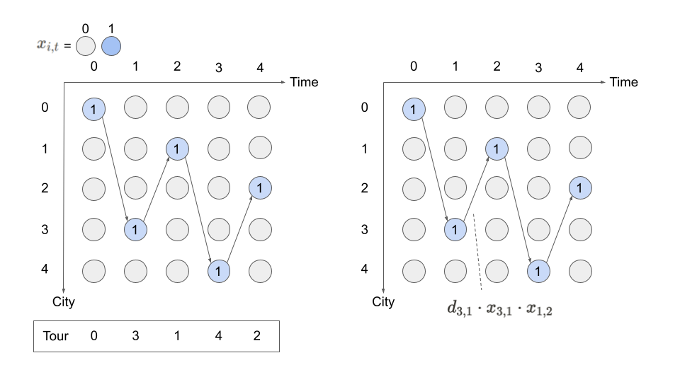
The following figure illustrates why these two constraints are needed for \(x_{i,t}\) to represent a tour.
Objective function#
The total distance of the tour, which is an objective function to be minimized, can be written as follows using the product of \(x\) representing the edges used between \(t\) and \(t+1\).
where \(d_{i, j} \geq 0\) is a distance between city \(i\) and city \(j\). “\(\mod n\)” is used to include in the sum the distance from the last city visited back to the first city visited. For example, when \(n\) is equal to 5 and node \(0\) is the first city visited, \(x_{0, (4+1)\mod 5}\) means \(x_{0, 0}\).
\(n\)-city TSP.#
where \(d_{i,j}\) is distance between city \(i\) and city \(j\).
Modeling by JijModeling#
Next, we show an implementation using JijModeling. We first define variables for the mathematical model described above.
import jijmodeling as jm

# define variables
d = jm.Placeholder('d', ndim=2)
N = d.len_at(0, latex="N")
i = jm.Element('i', belong_to=(0, N))
j = jm.Element('j', belong_to=(0, N))
t = jm.Element('t', belong_to=(0, N))
x = jm.BinaryVar('x', shape=(N, N))
d is a two-dimensional array representing the distance between each city.
N denotes the number of cities. This can be obtained from the number of rows in d.
i, j and t are subscripts used in the mathematical model described above.
Finally, we define the binary variable x to be used in this optimization problem.
# set problem
problem = jm.Problem('TSP')
problem += jm.sum([i, j], d[i, j] * jm.sum(t, x[i, t]*x[j, (t+1) % N]))
problem += jm.Constraint("one-city", x[:, t].sum() == 1, forall=t)
problem += jm.Constraint("one-time", x[i, :].sum() == 1, forall=i)
jm.sum([i, j], d[i, j] * jm.sum(t, x[i, t]*x[j, (t+1) % N])) represents objective function \(\sum_{i,j,t} d_{i, j}x_{i, t}x_{j, (t+1)\mod n}\).
The following jm.Constraint("one-city", x[:, t] == 1, forall=t) represents a constraint to visit one city at one time.
x[:, t] allows us to express \(\sum_i x_{i, t}\) concisely.
We can check the implementation of the mathematical model on the Jupyter Notebook.
problem
Prepare an instance#
We prepare the number of cities and their coordinates.
Here we select a metropolitan area in Japan using geocoder.
%%capture

# Install the required library
%pip install geopy
from geopy.geocoders import Nominatim
import numpy as np

geolocator = Nominatim(user_agent='python')

# set the name list of traveling points
points = ['Ibaraki', 'Tochigi', 'Gunma', 'Saitama', 'Chiba', 'Tokyo', 'Kanagawa']

# get the latitude and longitude
latlng_list = []
for point in points:
    location = geolocator.geocode(point)
    if location is not None:
        latlng_list.append([ location.latitude, location.longitude ])
# make distance matrix
num_points = len(points)
inst_d = np.zeros((num_points, num_points))
for i in range(num_points):
    for j in range(num_points):
        a = np.array(latlng_list[i])
        b = np.array(latlng_list[j])
        inst_d[i][j] = np.linalg.norm(a-b)
# normalize distance matrix
inst_d = (inst_d-inst_d.min()) / (inst_d.max()-inst_d.min())

geo_data = {'points': points, 'latlng_list': latlng_list}
instance_data = {'d': inst_d}
Solve by JijZeptSolver#
We solve this problem using jijzept_solver.
import jijzept_solver

interpreter = jm.Interpreter(instance_data)
instance = interpreter.eval_problem(problem)
solution = jijzept_solver.solve(instance, time_limit_sec=1.0)
Visualize the solution#
Using the solution obtained, we visualize the order of that salesman’s visit.
import matplotlib.pyplot as plt

df = solution.decision_variables_df
x_indices = df[df["value"] == 1.0]["subscripts"]
tour = [index for index, _ in sorted(x_indices, key=lambda x: x[1])]
tour.append(tour[0])

position = np.array(geo_data['latlng_list']).T[[1, 0]]

plt.axes().set_aspect('equal')
plt.plot(*position, "o")
plt.plot(position[0][tour], position[1][tour], "-")
plt.show()

print(np.array(geo_data['points'])[tour])
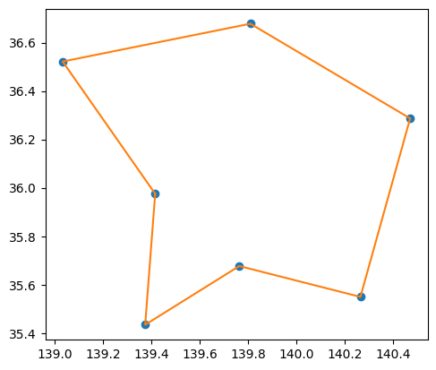
['Saitama' 'Gunma' 'Tochigi' 'Ibaraki' 'Chiba' 'Tokyo' 'Kanagawa'
 'Saitama']