Deep Space Network Scheduling#
Introduction: Deep Space Network (DSN)#
NASA’s Deep Space Network (hereafter referred to as DSN) is a network of radio telescopes.
These sites are Australia, Spain, and the United States.
These radio telescopes are used primarily for communication with spacecraft launched into space and for planetary observation missions in the radio wavelength band.
With the increasing number and complexity of spacecraft, communication scheduling with spacecraft is an extremely difficult problem.
In recent years, radio interferometry, a technique that uses interference between signals by networking multiple radio telescopes and manipulating them according to a pattern, has attracted much attention.
The most notable example is Event Horizon Telescope, which took the direct imaging of the supermassive black hole at the center of M87 and the Milky Way Galaxy.
Guillaume et al. (2022) formulated the DNS scheduling problem into QUBO and solved it using D-Wave’s hybrid solver.
Here, we implement this problem using JijModeling and solve it with JijZeptSolver.
DSN scheduling problem#
Problem setting#
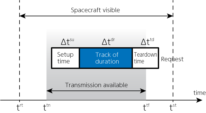
A schedule is generated after processing \(N\) requests \(\mathcal{Q} = \{Q_1, Q_2, \dots, Q_N\}\). A given request \(Q_n\) can utilize any of the \(M\) resources (antennas or equipments) prescribed for this request \(\mathcal{S} = \{S_1, S_2, \dots, S_M\}\). In turn, periods of visibility of a spacecraft from a particular ground station are calculated and define a set of \(K\) view periods \(\mathcal{V} = \{V_1, V_2, \dots, V_K \}\) for each resource \(S_m\). The times when a spacecraft becomes visible or invisible, respectively, the rise and set times, \(t^\mathrm{rt}\) and \(t^\mathrm{st}\), define the outer boundaries of a view period. The transmission to the spacecraft can begin (end) slightly later (earlier) than the rise and set time (respectively). These transmission on and off times, \(t^\mathrm{tn}\) and \(t^\mathrm{tf}\), delimit the inner boundaries within which a track can be scheduled. For each request, a setup and tear-down time period, \(\Delta t^\mathrm{su}\) and \(\Delta t^\mathrm{td}\), are given to prepare and remove (respectively) the equipment requested. Those times can occur anywhere between the rise and set times. In addition, a track duration \(\Delta t^\mathrm{dr}\) is prescribed for each request. An activity is defined as the period of time equal to the sum of the setup, track, and tear-down times, \(\Delta t^\mathrm{su}+\Delta t^\mathrm{dr}+\Delta t^\mathrm{td}\). It is the period of time during which an antenna can track a spacecraft and communicate with it. The goal of DSN schedule optimization is to process all requests; in other words, to schedule exactly one action per request. To this end, we use binary variables \(x_{n, m, k, t}\). These are equal to 1 when a track starts at time \(t\) within the view period \(k\) calculated for resource \(m\) of request \(n\), and \(0\) otherwise.
Constraint 1: Each request must be processed by one of the resources#
Each request must be processed by one of the resources. The request must be completed by \(t^\mathrm{tf}- \Delta t^\mathrm{dr}\) from the time \(t^\mathrm{tn}\) actually starts sending the request. The tracking time \(\Delta t^\mathrm{dr}\) must be taken into account.
Constraint 2: Avoiding conflicts#
In addition, the schedule should be devoid of conflicts as the figure below.
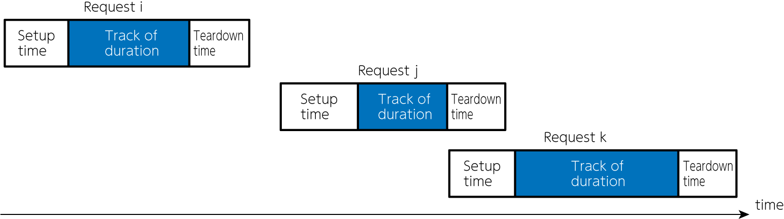
The figure shows requests \(i\) and \(j\), \(i\) and \(k\) do not conflict, but \(j\) and \(k\) overlap, indicating that they are in conflict. We have to avoid such conflicts. This can be expressed in the formula as follows:
Implementation#
Here, we implement a script that solve this problem using JijModeling and JijZeptSolver.
Define variables#
We define the variables for eq.(1) and (2).
import jijmodeling as jm

# define variables
AT = jm.Placeholder('AT', ndim=4)
max_AT = jm.Placeholder('max_AT')
N = jm.Placeholder('N')
M = jm.Placeholder('M')
K = jm.Placeholder('K')
su = jm.Placeholder('su', ndim=1)
dr = jm.Placeholder('dr', ndim=1)
td = jm.Placeholder('td', ndim=1)
x = jm.BinaryVar('x', shape=(N, M, K, max_AT))
n1 = jm.Element('n1', belong_to=N)
n2 = jm.Element('n2', belong_to=N)
m = jm.Element('m', belong_to=M)
k1 = jm.Element('k1', belong_to=K)
k2 = jm.Element('k2', belong_to=K)
t1 = jm.Element('t1', belong_to=AT[n1, m, k1])
t2 = jm.Element('t2', belong_to=AT[n2, m, k2])
AT is the starting time of processing requests, max_AT is the maximum value of AT, N is the number of requests, M is the number of ground resources, and K is the number of viewperiods.
su, dr, and td are the setup time \(\Delta t^\mathrm{su}\), tracking duration \(\Delta t^\mathrm{dr}\), and teardown time \(\Delta t^\mathrm{td}\) for each request, respectively.
Also, we define binary variables x and the subscripts used to represent \(x_{n, m, k, t}\) as n1, n2, m, k1, k2, t1, t2.
The possible ranges of the subscripts t1 and t2 are described as AT[n1, m, k1], AT[n2, m, k2].
In other word, \(t_1 \in \mathrm{AT}_{n1, m, k1}, t_2 \in \mathrm{AT}_{n2, m, k2}\).
Implement the mathematical model#
Then, we implement eq.(1) and (2) as constraints.
# make problem
problem = jm.Problem('Radio_telescope_scheduling')
# set constraint 1: onehot constraint
problem += jm.Constraint('onehot', jm.sum([m, k1, t1], x[n1, m, k1, t1])==1, forall=n1)
# set constraint 2: avoid conflict
problem += jm.Constraint('conflict', x[n1, m, k1, t1]*x[n2, m, k2, t2]==0,
                         forall=[n1, (n2, n2!=n1), m, k1, k2, t1,
                                 (t2, (t1-su[n1]<=t2-su[n2]) & (t2-su[n2]<=t1+dr[n1]+td[n1]) | ((t2-su[n2]<=t1-su[n1]) & (t1-su[n1]<=t2+dr[n2]+td[n2])))])
The \(\sum_{m, k, t}\) in equation (1) is written as sum([m, k, t], ...) .
To represent all \(n_1, n2\) combinations except \(n_1 \neq n2\) in equation (2), we use forall=[n1, (n2, n2!=n1)].
\(t_{n1} - \Delta t^\mathrm{su}_{n1} \leq t_{n2} - \Delta t^\mathrm{su}_{n2} \leq t_{n1} + \Delta t^\mathrm{dr}_{n1} + \Delta t^\mathrm{td}_{n1}\) is then expressed as forall=[t1, (t2, (t1-su[n1]<=t2-su[n2]) & (t2-su[n2]<=t1+dr[n1]+td[n1]))] using AND operator.
To impose multiple conditions on a given index, we can use the AND operator & and the OR operator |.
With Jupyter Notebook, we can check the mathematical model implemented.
problem
Prepare an instance#
Next, we create an instance.
import collections
import numpy as np

def flatten(l):
    for el in l:
        if isinstance(el, collections.abc.Iterable) and not isinstance(el, (str, bytes)):
            yield from flatten(el)
        else:
            yield el

# set the number of requests
inst_N = 12
# set a list of set up time period: su
rng = np.random.default_rng(1234)
inst_su = rng.normal(2.0, 0.5, inst_N)
# set a list of track duration: dr
inst_dr = rng.normal(2.0, 0.5, inst_N)
# set a list of tear down time period: td
inst_td = rng.normal(1.5, 0.5, inst_N)
# set a array of transmission-on time: tn
inst_tn = np.array([[0, 6, 12, 18], [2, 8, 14, 20], [4, 10, 16, 22]])
# set a array of transmission-off time: tf
inst_tf = np.array([[4, 10, 16, 22], [6, 12, 18, 24], [8, 14, 20, 26]])
# get the number of resources and viewperiods
inst_M = inst_tn.shape[0]
inst_K = inst_tn.shape[1]
# compute a array of available time tn ≤ t ≤ tf - dr
inst_available = []
for n in range(inst_N):
    inst_available.append([])
    for i in range(inst_M):
        inst_available[n].append([])
        for j in range(inst_tf.shape[1]):
            inst_available[n][i].append(list(range(inst_tn[i, j], np.floor(inst_tf[i, j]-inst_dr[n]).astype(int))))
# compute max(available time)
inst_max_available = np.amax(list(flatten(inst_available))) + 1
instance_data = {'AT': inst_available, 'su': inst_su, 'dr': inst_dr, 'td': inst_td, 'max_AT': inst_max_available, 'N': inst_N, 'M': inst_M, 'K': inst_K}
Solve by JijZeptSolver#
We solve this problem using jijzept_solver.
import jijzept_solver

interpreter = jm.Interpreter(instance_data)
instance = interpreter.eval_problem(problem)
solution = jijzept_solver.solve(instance, time_limit_sec=1.0)
Visualize the solution#
Then, we visualize the solution obtained.
import matplotlib.pyplot as plt
import matplotlib.ticker as ticker

df = solution.decision_variables_df
x_indices = np.array(df[df["value"]==1]["subscripts"].to_list())
n_indices = x_indices[:, 0]
m_indices = x_indices[:, 1]
k_indices = x_indices[:, 2]
t_indices = x_indices[:, 3]
# make plot
fig, ax = plt.subplots()
# set x- and y-axis
ax.set_xlabel("Time")
ax.set_yticks(range(inst_M))
ax.set_yticklabels(["Resource {}".format(m) for m in range(inst_M)])
ax.get_xaxis().set_major_locator(ticker.MaxNLocator(integer=True))
# make bar plot for transmission using broken_barh
for n, m, k, t in zip(n_indices, m_indices, k_indices, t_indices):
    ax.broken_barh([(t, inst_dr[n])], (m-0.5, 1), color="dodgerblue")
    ax.broken_barh([(t-inst_su[n], inst_su[n])], (m-0.5, 1), color="gold")
    ax.broken_barh([(t+inst_dr[n], inst_td[n])], (m-0.5, 1), color="violet")
# make bar plot for available time
for m, (list_tn, list_tf) in enumerate(zip(inst_tn, inst_tf)):
    for tn, tf in zip(list_tn, list_tf):
        ax.broken_barh([(tn, tf-tn-1)], (m-0.5, 1), color="lightgray", alpha=0.4)
# make legend
ax.scatter([], [], color="lightgray", label="Transimission available", marker="s")
ax.scatter([], (), color="dodgerblue", label="Tracking", marker="s")
ax.scatter([], (), color="gold", label="Set up", marker="s")
ax.scatter([], (), color="violet", label="Tear down", marker="s")
ax.legend(bbox_to_anchor=(1.45, 1.0))
# show plot
plt.show()
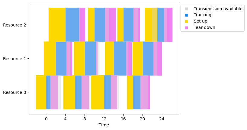
The gray regions indicate the times when each resource can communicate with the satellite. The blue bands represent the tracking. The yellow and magenta colors represent the setup time and teardown time for each request, respectively. We can see that all tracking durations overlap the gray communication available time.