The K-Median Problem

The k-median problem is the problem of clustering data points into k clusters, aiming to minimize the sum of distances between points belonging to a particular cluster and the data point that is the center of the cluster. This can be considered a variant of k-means clustering. For k-means clustering, we determine the mean value of each cluster, whereas for k-median we use the median value. This problem is known as NP-hard. We describe how to implement the mathematical model of k-median problem with JijModeling and solve it with JijZept.

Mathematical Model

Let us consider a mathematical model for k-median problem.

Decision variables

We denote \(x_{i, j}\) to be a binary variable which is 1 if \(i\)-th data point belongs to the \(j\)-th median data point and 0 otherwise. We also use a binary variable \(y_j\) which is 1 if \(j\)-th data point is the median and 0 otherwise.

\[\begin{split} x_{i,j} = \begin{cases} 1,~\text{Node $i$ is covered by median $j$}\\ 0,~\text{Otherwise} \end{cases} \end{split}\]

\[\begin{split} y_j = \begin{cases} 1,~\text{Node $j$ is a median.}\\ 0,~\text{Otherwise} \end{cases} \end{split}\]

Mathematical Model

Our goal is to find a solution that minimizes the sum of the distances between \(i\)-th data point and \(j\)-th median point. We also set three constraints:

1. A data point must belong to a single median data point,

2. The number of median points is \(k\),

3. The data points must belong to a median point.

These can be expressed in a mathematical model as follows.

\[\begin{split} \begin{aligned} \min_x &\sum_{i}\sum_j d_{i,j}x_{i,j} \\ \mathrm{s.t.}~&\sum_{j} x_{i,j} = 1,~\forall i\\ &\sum_j y_j = k\\ &x_{i,j} \leq y_j, ~\forall i, j\\ &x_{i,j} \in \{0, 1\} ~\forall i, j\\ &y_j \in \{0, 1\}~\forall j \end{aligned} \tag{1} \end{split}\]

Modeling by JijModeling

Here, we show an implementation using JijModeling. We first define variables for the mathematical model described above.

import jijmodeling as jm

d = jm.Placeholder("d", ndim=2)
N = d.len_at(0, latex="N")
J = jm.Placeholder("J", ndim=1)
k = jm.Placeholder("k")
i = jm.Element("i", belong_to=(0, N))
j = jm.Element("j", belong_to=J)
x = jm.BinaryVar("x", shape=(N, J.shape[0]))
y = jm.BinaryVar("y", shape=(J.shape[0],))

d is a two-dimensional array representing the distance between each data point and the median point. The number of data points N is extracted from the number of elements in d. J is a one-dimensional array representing the candidate indices of the median point. k is the number of median points. i and j denote the indices used in the binary variables, respectively. Finally, we define the binary variables x and y.

Then, we implement equations (1).

problem = jm.Problem("k-median")
problem += jm.sum([i, j], d[i, j]*x[i, j])
problem += jm.Constraint("onehot", x[i, :].sum() == 1, forall=i)
problem += jm.Constraint("k-median", y[:].sum() == k)
problem += jm.Constraint("cover", x[i, j] <= y[j], forall=[i, j])

With jm.Constraint("onehot", x[i, :].sum() == 1, forall=i), we insert as a constraint that \(\sum_j x_{i, j} = 1\) for all \(i\). jm.Constraint("k-median", y[:].sum() == k) represents \(\sum_j y_j = k\). jm.Constraint("cover", x[i, j] <= y[j], forall=[i, j]) requires that \(x_{i, j} \leq y_j\) must be for all \(i, j\).

We can check the implementation of the mathematical model on Jupyter Notebook.

problem

\[\begin{split}\begin{array}{cccc}\text{Problem:} & \text{k-median} & & \\& & \min \quad \displaystyle \sum_{i = 0}^{N - 1} \sum_{j \in J} d_{i, j} \cdot x_{i, j} & \\\text{{s.t.}} & & & \\ & \text{cover} & \displaystyle x_{i, j} \leq y_{j} & \forall i \in \left\{0,\ldots,N - 1\right\} \forall j \in J \\ & \text{k-median} & \displaystyle \sum_{\ast_{0} = 0}^{\mathrm{len}\left(J, 0\right) - 1} y_{\ast_{0}} = k & \\ & \text{onehot} & \displaystyle \sum_{\ast_{1} = 0}^{\mathrm{len}\left(J, 0\right) - 1} x_{i, \ast_{1}} = 1 & \forall i \in \left\{0,\ldots,N - 1\right\} \\\text{{where}} & & & \\& y & 1\text{-dim binary variable}\\& x & 2\text{-dim binary variable}\\\end{array}\end{split}\]

Prepare instance

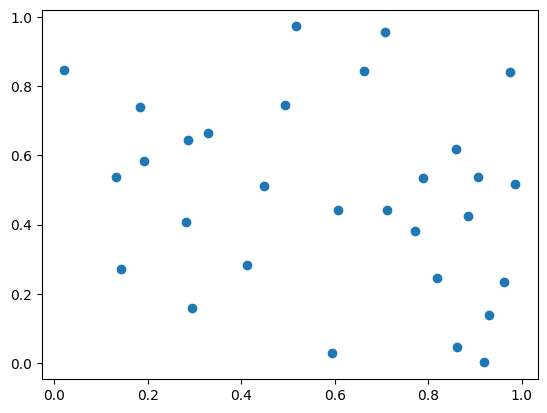
We prepare and visualize data points.

import matplotlib.pyplot as plt
import numpy as np

num_nodes = 30
X, Y = np.random.uniform(0, 1, (2, num_nodes))

plt.plot(X, Y, "o")

[<matplotlib.lines.Line2D at 0x7fc02c0dccd0>]

We compute the distance between each data point.

XX, XX_T = np.meshgrid(X, X)
YY, YY_T = np.meshgrid(Y, Y)
inst_d = np.sqrt((XX - XX_T)**2 + (YY - YY_T)**2)
inst_J = np.arange(0, num_nodes)
inst_k = 4
instance_data = {"d": inst_d, "J": inst_J, "k": inst_k}

Solve with JijSolver

We solve the problem using jijsolver.

import jijsolver
 
interpreter = jm.Interpreter(instance_data)
instance = interpreter.eval_problem(problem)
solution = jijsolver.solve(instance, time_limit_sec=1.0)

Visualize the solution

We visualize the solution obtained/

df = solution.decision_variables
y_indices = np.ravel(df[(df["name"] == "y") & (df["value"] == 1.0)]["subscripts"].to_list())
x_indices = df[(df["name"] == "x") & (df["value"] == 1.0)]["subscripts"].to_list()

median_X, median_Y = X[y_indices], Y[y_indices]
d_from_m = np.sqrt((X[:, None]-X[y_indices])**2 + (Y[:, None]-Y[y_indices])**2)
cover_median = y_indices[np.argmin(d_from_m, axis=1)]
plt.plot(X, Y, "o")
plt.plot(X[y_indices], Y[y_indices], "o", markersize=10)
plt.plot(np.column_stack([X, X[cover_median]]).T, np.column_stack([Y, Y[cover_median]]).T, c="gray")
plt.show()

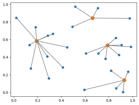
This figure shows how they are in clusters. Orange and blue points show the median and other data points, respectively. The gray line connects the median and the data points belonging to that cluster.