An optimization for preventing a pandemic on a university campus

Introduction: How to prevent pandemics using a combinatorial optimization?

The pandemic of COVID-19, which began worldwide at the end of 2019, has changed people’s lives. The pandemic resulted in temporary restrictions on admission to the campus for college students. Sud & Li (2021) introduced a recursive approach to the Max-Cut problem using quantum annealing to map groups of students on college campuses into cohorts and showed a result of preventing infection spread. In this tutorial, we use JijModeling and JijSolver for implementing this algorithm. We also solve an actual infection model from that cohort and see how much the infection spreads.

Algorithm for making cohorts

By dividing students into several groups, separating the days they come to campus and the classrooms they use, to prevent the spread of infection. To do this, we consider the connections between students as a graph. We solve that graph as the Max-Cut problem, and divide it into two parts.

We repeat solving the Max-Cut problem until we get the desired number of cohorts, at which point we end the iteration.

G = Network Graph
N = Target number of cohorts (power of 2)
currCohorts = [G]
while currCohorts.length < N do
    newCohorts = []
    for c in currCohorts do
        c1, c2 = performMaxcut(c)
        newCohorts.append(c1)
        newCohorts.append(c2)
    end
    currCohorts = newCohorts
end

performMaxcut function, which we describe and implement later, is a function that solves the maximum cut problem and splits the graph into two parts. Sud & Li (2021) use a D-Wave quantum annealer. Here, we implement performMaxcut using JijModeling and JijSolver.

A mathematical model for the Max-Cut optimization

To partition a graph \(G = (V, E)\) into two subgraphs, we solve the Max-Cut problem. In the following, we consider its formulation. We divide the vertices belonging to \(G\) into two sets, positive and negative. The problem is to find the division such that the sum of the weights of the cut edges is maximized.

Ensure that the weight of the cut edge is maximized

We use spin variables such that \(s_i = 1\) when vertex \(i\) belongs to the positive set and \(s_i = -1\) vice versa. Next, we consider the sum of the cut edges to have maximum weight. We represent the weight that the edge connecting vertex \(i\) and vertex \(j\) as \(w_{ij}\). Since we consider only the vertices belonging to the positive vertices set and the negative sets, the sum of them is written as follows.

\[ \mathrm{obj} = - \sum_{(i, j) \in E} \frac{w_{ij}}{2} (1-s_i s_j) \tag{1} \]

When \(s_i = s_j\), \(1-s_i s_j = 0\), which expresses that only the weights on the edges of \(s_i \neq s_j\) are added. We consider purely dividing the students into two groups. Therefore, we set \(w_{ij} = 1\) in this problem.

Conversion to binary variables

Since JijModeling only supports binary variables, we have to consider the correspondence with spin variables. Let us consider binary variables such that \(x_i = 1\) when the vertex \(i\) belongs to the positive set and \(x_i = -1\) vice versa. Then the correspondence between \(s_i\) and \(x_i\) is

\[ x_i = \frac{1+s_i}{2} \ \Longrightarrow \ s_i = 2 x_i - 1 \tag{2} \]

Let’s code!

Here, we implement a script that solves this problem using JijModeling and JijSolver.

Defining variables

We define the variables for the Max-Cut problem as follows.

import jijmodeling as jm

# define variables
V = jm.Placeholder('V')
E = jm.Placeholder('E', ndim=2)
w = jm.Placeholder('w', ndim=2)
x = jm.BinaryVar('x', shape=(V, ))
e = jm.Element('e', belong_to=E)
i = jm.Element('i', belong_to=V)
j = jm.Element('j', belong_to=V)

V, E, w, and x denote the number of graph vertices, the edge set, the graph weights, and binary variables, respectively. e, i and j are varibles for indices.

Implementation for the Max-Cut problem

Next, we implement the objective function (1) for the Max-Cut problem.

# make problem
problem = jm.Problem('Max cut')
# set spin variables
si = 2 * x[e[0]] - 1
sj = 2 * x[e[1]] - 1
# set objective function: maximize the cut-edge weights
obj = - jm.sum(e, 0.5*w[e[0], e[1]]*(1-si*sj))
problem += obj

First, we define two spin variables, and then we implement equation (1).
With Jupyter Notebook, we can check the mathematical model implemented.

problem

\[\begin{split}\begin{array}{cccc}\text{Problem:} & \text{Max cut} & & \\& & \min \quad \displaystyle - \sum_{e \in E} 0.5 \cdot w_{e_{0}, e_{1}} \cdot \left(- \left(2 \cdot x_{e_{0}} - 1\right) \cdot \left(2 \cdot x_{e_{1}} - 1\right) + 1\right) & \\\text{{where}} & & & \\& x & 1\text{-dim binary variable}\\\end{array}\end{split}\]

Preparing the Networks

We create a graph that imitates a network formed by multiple people, such as on a college campus. Here we adopt the small-world graph proposed in Watts & Strogatz(1998).

import networkx as nx

# set a small-world graph
inst_V = 1000
k = 20
p = 0.1
inst_G = nx.watts_strogatz_graph(inst_V, k, p)
# set weights on the edges
for edge in inst_G.edges:
    inst_G[edge[0]][edge[1]]['weight'] = 1.0

Solving with JijSolver

We solve the Max-Cut problem using jijsolver. We write functions for iteratively performing the Max-Cut optimization.

import jijsolver
import numpy as np

# A function to prepare a graph instance for MaxCut
def make_instance(input_c):
    # get the number of nodes
    inst_V = len(input_c.nodes)
    # relavel name of nodes
    mapping_dict = {a: b for a, b in zip(input_c.nodes, range(inst_V))}
    c = nx.relabel_nodes(input_c, mapping_dict)
    # get edges and weights
    inst_E = [[edge[0], edge[1]] for edge in c.edges]
    inst_w = np.zeros([inst_V, inst_V])
    for k, v in nx.get_edge_attributes(c, 'weight').items():
        inst_w[k[0], k[1]] = v
    return {'V': inst_V, 'E': inst_E, 'w': inst_w}

# A function to make two graphs from JijZept results
def make_graph(solution, c):
    df = solution.decision_variables
    x_indices = np.ravel(df[df["value"]==1]["subscripts"].to_list())
    # extract a subgraph (x=1) from original graph
    c1 = c.copy()
    c1 = c1.subgraph(x_indices)
    # remove a subgraph from the original graph
    c2 = c.copy()
    c2.remove_nodes_from(x_indices)
    return c1, c2

# execute MaxCut
def performMaxcut(c):
    instance_data = make_instance(c)
    # compute the Max-Cut using JijSolver
    interpreter = jm.Interpreter(instance_data)
    instance = interpreter.eval_problem(problem)
    solution = jijsolver.solve(instance, time_limit_sec=1.0)
    return make_graph(solution, c)

We solve the Max-Cut problem iteratively using the functions described above.

# set the number of cohorts
N = 4
currCohorts = [inst_G, ]
# iteration
while len(currCohorts) < N:
    newCohorts = []
    for c in currCohorts:
        c1, c2 = performMaxcut(c)
        newCohorts.extend([c1, c2])
    currCohorts = newCohorts

This calculation yields N graphs.

Input to the SIR epidemic model

The SIR model, introduced by Kermack & McKendrick (1927), is one of the well-known models of infectious diseases. It consists of the following three differential equations:

\[ \frac{dS}{dt} = -\beta S I \tag{3} \]

\[ \frac{dI}{dt} = \beta S I - \gamma I \tag{4} \]

\[ \frac{dR}{dt} = \gamma I \tag{5} \]

where \(S\) is susceptible (but not yet infected with the disease), \(I\) is the number of infectious and \(R\) is the number of individuals who recovered from the disease. The parameters \(\beta\) and \(\gamma\) are constants that represent the infection and recovery rates, respectively. In COVID-19, the average recovery period is known to be \(Tr\) = 10 days, so \(\gamma = 1/ Tr\). Also, we write the average number of people who transfer the infection while infected as \(\alpha\). It can be written as:

\[ \alpha = \mathrm{avg\_deg}(G) \times \frac{\beta}{\gamma} \tag{6} \]

where \(\mathrm{avg\_deg}(G)\) denotes the degree of the average of the graph \(G\). \(\alpha\) value for COVID-19 has been reported to range from 1.5 to 6.7. Using a chosen \(\alpha\) value, we can estimate \(\beta\) via equation (6). By solving the SIR model equation in connection with the graph of student connections, we can model how infectious diseases spread on the campus. Now, let us input the cohort of students divided by the above algorithm into this model and see how the number of infections changes. Here, we will use NDlib library, which has the function to solve the SIR model that can take into account the graph topology.

import ndlib.models.ModelConfig as mc
import ndlib.models.epidemics as ep

# a function for solving the SIR model
def solveSIR(g):
    # compute the average degree of a graph
    list_degree = [g.degree[n] for n in g.nodes()]
    avg_deg = sum(list_degree) / len(list_degree)
    # set parameters for SIR model
    gamma = 1.0 / 10
    alpha = 3.0
    beta = alpha * gamma / avg_deg
    # set SIR model
    model = ep.SIRModel(g)
    # input parameters
    cfg = mc.Configuration()
    cfg.add_model_parameter('beta', beta)
    cfg.add_model_parameter('gamma', gamma)
    cfg.add_model_parameter('percentage_infected', 0.05)
    model.set_initial_status(cfg)
    # compute the SIR model
    iterations = model.iteration_bunch(100)
    trends = model.build_trends(iterations)
    return model, trends

For comparison, the following is a visualization of the computation results with MaxCut and a randomly separated graph.

from ndlib.viz.mpl.DiffusionTrend import DiffusionTrend
from ndlib.viz.mpl.TrendComparison import DiffusionTrendComparison
import random

# solve the SIR model
model1, trends1 = solveSIR(currCohorts[0])

cohort_idx = 0
list_random_partition_nodes = []
for i in inst_G.nodes:
    if random.randint(0, N-1) == cohort_idx:
        list_random_partition_nodes.append(i)
G_temp = inst_G.copy()
random_g = G_temp.subgraph(list_random_partition_nodes)
# solve the SIR model
model2, trends2 = solveSIR(random_g)

viz = DiffusionTrendComparison([model1, model2], [trends1, trends2], "Infected")
viz.plot()

no display found. Using non-interactive Agg backend
no display found. Using non-interactive Agg backend

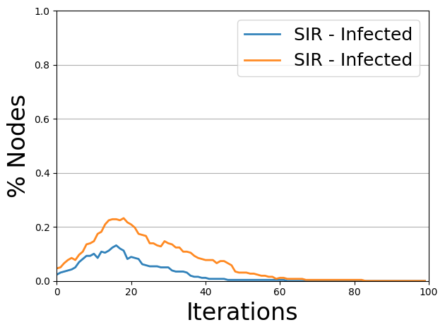
The blue line indicates the number of infected cases with MaxCut, and the orange line shows the number of infected cases with random separation. We can see that the MaxCut scenario is lower than the random one. We embed the actual human contacts into a graph and partition according to this method. Then, we change the day of school attendance on campus for each group created by the partitioning, we prevent the pandemic.

References

• Sud & Li, 2021, “A Quantum Annealing Approach to Reduce Covid-19 Spread on College Campuses”

• Watts & Strogatz, 1998, “Collective dynamics of ‘small-world’ networks”

• Kermack & McKendrick, 1927, “A contribution to the mathematical theory of epidemics”

• Rossetti et al., 2017, “NDLIB: a python library to model and analyze diffusion processes over complex networks”