クリーク被覆問題

ここでは、JijSolverとJijModelingを用いて、クリーク被覆問題を解く方法を説明します。 この問題は、Lucas, 2014, “Ising formulations of many NP problems”の 6.2. Clique Coverでも触れられています。

クリーク被覆問題とは

この問題は、与えられたグラフを分割できる、クリーク (完全グラフ)の最少数を求めるというものです。 これはNP完全問題としても知られています。

完全グラフ

完全グラフとは、グラフ内の2頂点間がすべて辺で結ばれているようなグラフのことです (ただしループや多重辺は含まれません。) 例として、以下のようなものが挙げられます。

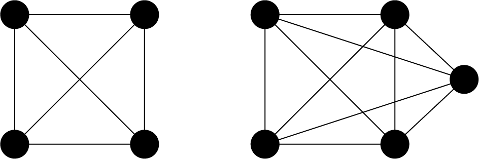
先程説明したように、完全グラフの頂点は、その他の全ての頂点と辺で結ばれています。 完全無向グラフ \(G = (V, E)\)は、\({}_V C_2 = \frac{1}{2} V (V-1)\)個の辺を持ちます。 すなわち、辺の数は頂点\(V\)の中から2つを選ぶ組合せの数となります。 完全グラフの辺数からのずれを最小化することで、クリーク被覆問題の数理モデルを記述してみましょう。

数理モデルの構築

最初に、もし頂点\(v\)が\(n\)番目の部分グラフに含まれるなら1、そうでないなら0となるようなバイナリ変数\(x_{v, n}\)を導入しましょう。

制約: 頂点は必ず1つのクリークに属さなければならない。

この問題では、各頂点は必ず1つのクリークに含まれる必要があります。

\[ \sum_{n=0}^{N-1} x_{v, n} = 1 \quad (\forall v \in V) \tag{1} \]

目的関数: 完全グラフの辺数からの差を最小化する

\(n\)番目の部分グラフ\(G (V_n, E_n)\)を考えましょう。 この部分グラフが完全グラフのとき、先程の議論から、この部分グラフの変数は\(\frac{1}{2} V_n (V_n - 1)\)となります。 これに対し、\(n\)番目の部分グラフの辺の数は\(\sum_{(uv) \in E_n} x_{u, n} x_{v, n}\)のように計算できます。 この2つの差が0に近いほど、その部分グラフはクリークに近くなります。 よって、この問題を目的関数は以下のようになります。

\[ \sum_{n=0}^{N-1} \left\{ \frac{1}{2} \left( \sum_{v=0}^{V-1} x_{v, n} \right) \left( \sum_{v=0}^{V-1} x_{v, n} -1\right) - \sum_{(uv) \in E} x_{u, n} x_{v, n} \right\} \tag{2} \]

JijModelingによるモデル化

次に、JijModelingを用いた実装を示します。 最初に、上述の数理モデルで用いる変数を定義しましょう。

import jijmodeling as jm

# define variables
V = jm.Placeholder('V')
E = jm.Placeholder('E', ndim=2)
N = jm.Placeholder('N')
x = jm.BinaryVar('x', shape=(V, N))
n = jm.Element('n', belong_to=(0, N))
v = jm.Element('v', belong_to=(0, V))
e = jm.Element('e', belong_to=E)

制約

次に、制約式(1)を実装しましょう。

# set problem
problem = jm.Problem('Clique Cover')
# set one-hot constraint: each vertex has only one color
problem += jm.Constraint('color', x[v, :].sum()==1, forall=v)

x[v, :].sum()は、sum(n, x[v, n])と同じ意味です。

目的関数

次に、目的関数式(2)を実装しましょう。

# set objective function: minimize the difference in the number of edges from a complete graph
clique = x[:, n].sum() * (x[:, n].sum()-1) / 2
num_e = jm.sum(e, x[e[0], n]*x[e[1], n])
problem += jm.sum(n, clique-num_e)

Jupyter Notebookで、実装された数理モデルを表示してみましょう。

problem

\[\begin{split}\begin{array}{cccc}\text{Problem:} & \text{Clique Cover} & & \\& & \min \quad \displaystyle \sum_{n = 0}^{N - 1} \left(\sum_{\ast_{0} = 0}^{V - 1} x_{\ast_{0}, n} \cdot \left(\sum_{\ast_{0} = 0}^{V - 1} x_{\ast_{0}, n} - 1\right) \cdot 2^{(-1)} - \sum_{e \in E} x_{e_{0}, n} \cdot x_{e_{1}, n}\right) & \\\text{{s.t.}} & & & \\ & \text{color} & \displaystyle \sum_{\ast_{1} = 0}^{N - 1} x_{v, \ast_{1}} = 1 & \forall v \in \left\{0,\ldots,V - 1\right\} \\\text{{where}} & & & \\& x & 2\text{-dim binary variable}\\\end{array}\end{split}\]

インスタンスの準備

Networkxを用いて、グラフを準備しましょう。

import networkx as nx

# set the number of colors
inst_N = 3
# set empty graph
inst_G = nx.Graph()
# add edges
inst_E = [[0, 1], [1, 2], [0, 2], 
            [3, 4], [4, 5], [5, 6], [3, 6], [3, 5], [4, 6], 
            [7, 8], [8, 9], [7, 9], 
            [1, 3], [2, 6], [5, 7], [5, 9]]
inst_G.add_edges_from(inst_E)
# get the number of nodes
inst_V = list(inst_G.nodes)
num_V = len(inst_V)
instance_data = {'N': inst_N, 'V': num_V, 'E': inst_E}

準備されたグラフを可視化してみましょう。

import matplotlib.pyplot as plt

nx.draw_networkx(inst_G, with_labels=True)
plt.show()

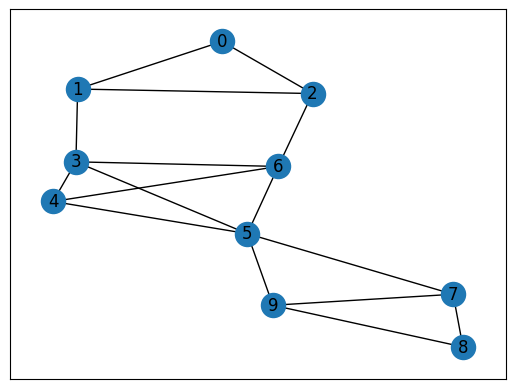
このグラフは、(0, 1, 2), (3, 4, 5, 6), (7, 8, 9)の3つのクリークからなることがわかります。 次は、JijSolverで解いてみましょう。

JijSolverで解く

この問題を、jijsolverで解きましょう。

import jijsolver

interpreter = jm.Interpreter(instance_data)
instance = interpreter.eval_problem(problem)
solution = jijsolver.solve(instance, time_limit_sec=1.0)

最後に、得られた解を可視化しましょう。

df = solution.decision_variables
x_indices = df[df["value"]==1.0]["subscripts"]
# initialize vertex color list
node_colors = [-1] * len(x_indices)
# set color list for visualization
cmap = plt.get_cmap("tab10")
colorlist = [cmap(i) for i in range(inst_N)]
# set vertex color list
for i, j in x_indices:
    node_colors[i] = colorlist[j]
# make figure
nx.draw_networkx(inst_G, node_color=node_colors, with_labels=True)
plt.show()

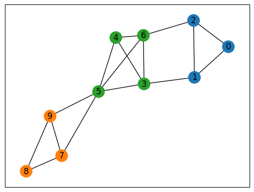
予想通り、JijSolverによりグラフを3つのクリークに分割することができました。