ハミルトニアンサイクル・経路問題

ここではJijSolverとJijModelingを用いて、ハミルトニアンサイクルとハミルトニアン経路問題を解く方法を説明します。 この問題は、Lucas, 2014, “Ising formulations of many NP problems” 7.1. Hamiltonian Cycles and Paths でも触れられています。

ハミルトニアンサイクル・経路とは

ハミルトニアン経路問題とは、グラフ内のある頂点から出発し、グラフの各頂点を1度だけ訪れながら全ての頂点を訪れるような経路を求める問題です。 加えて、ハミルトニアンサイクル問題は、最初に出発した頂点に帰ってくるようにしたものです (すなわち、最初に出発した頂点だけ2回訪れることになります。) この問題は、有向・無向のどちらのグラフも考えることができます。

数理モデル

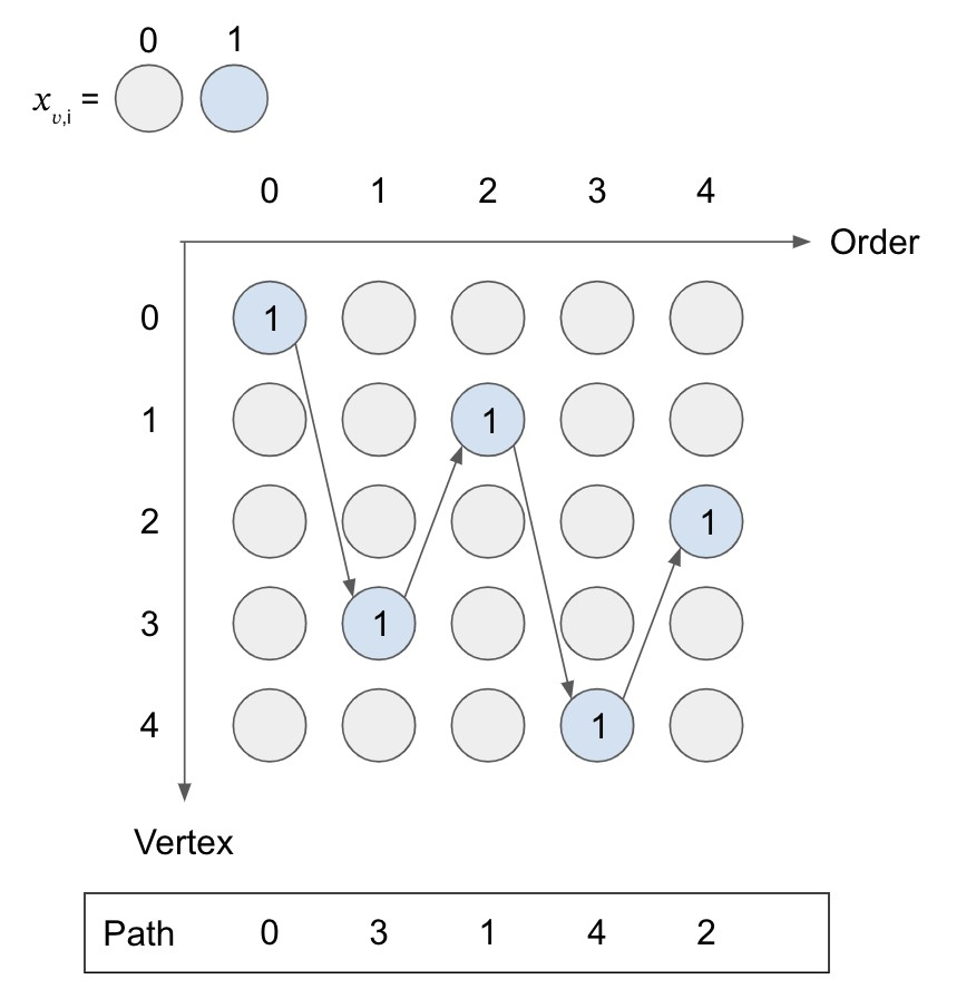
一般性を失うことなく、頂点に\(1, \cdots, V\)のようにラベルをつけ、さらにグラフの辺が有向であるとしましょう。 すなわち辺\((uv)\)と辺\((vu)\)は、異なる辺であるとします。 与えられたグラフ\(G = (V, E)\)において、\(i\)番目に頂点\(v\)を訪れるとき1、そうでないとき0となるようなバイナリ変数\(x_{v, i}\)を導入しましょう。

制約 1: 全ての頂点を1回だけ訪れなければならない

この制約は、次のように簡潔に定式化することができます。

\[ \quad \sum_{i=1}^V x_{v, i} = 1 \quad \text{for } v = 1, \cdots , V. \]

制約 2: 経路は繋がっていなければならない

これは、\(i\)番目に訪れる頂点は1つだけでなければならないことを意味します。

\[ \quad \sum_{v=1}^V x_{v, i} = 1 \quad \text{for } i = 1, \cdots , V. \]

下図は、有効な経路を示したものです。 各行・各列で1の値をとる変数の数を数えることで、制約1・2の条件が成立していることを確認することができます。

制約 3: 経路に用いられる辺\((u, v)\)は、\(G\)内に存在しなければならない

経路に辺\((u, v)\)を用いる場合、\(x_{u, i}\)と\(x_{v, i+1}\)は1でなければなりません。 これを数式で表すと、次のようになります。

\[ \quad \sum_{(u,v) \notin E} \sum_{i=1}^{V} x_{u,i} x_{v, (i+1)\%V} = 0 \]

ここで示した制約は、ハミルトニアンサイクル問題のためのものです。 ハミルトニアン経路問題を考える場合には、代わりに\(\sum_{i=1}^V\) to \(\sum_{i=1}^{V-1}\)のような制約を考える必要があります。 これは、最初に出発する頂点と最後に訪れる頂点の間の辺について考慮する必要がないことを意味します。

JijModelingによるモデル化

JijModelingを用いて、上述の方程式を実装する方法を説明します。 まずは、数理モデルで必要な変数を定義していきましょう。

import jijmodeling as jm

# define variables
V = jm.Placeholder('V')
barE = jm.Placeholder('barE', ndim=2)
num_barE = barE.shape[0]
i = jm.Element('i', V)
v = jm.Element('v', V)
x = jm.BinaryVar('x', shape=(V, V))
f = jm.Element('f', num_barE)

3つの制約を、次のように実装します。

problem = jm.Problem("Hamiltonian Cycles")
problem += jm.Constraint('one-vertex', x[v, :].sum()==1, forall=v)
problem += jm.Constraint('one-path', x[:, i].sum()==1, forall=i)
problem += jm.Constraint('one-edge', jm.sum([f,i], x[barE[f][0],i]*x[barE[f][1],(i+1)%V])==0)

Jupyter Notebook上で、実装した問題を表示してみましょう。

problem

\[\begin{split}\begin{array}{cccc}\text{Problem:} & \text{Hamiltonian Cycles} & & \\& & \min \quad \displaystyle 0 & \\\text{{s.t.}} & & & \\ & \text{one-edge} & \displaystyle \sum_{f = 0}^{\mathrm{len}\left(barE, 0\right) - 1} \sum_{i = 0}^{V - 1} x_{barE_{f, 0}, i} \cdot x_{barE_{f, 1}, \left(i + 1\right) \bmod V} = 0 & \\ & \text{one-path} & \displaystyle \sum_{\ast_{0} = 0}^{V - 1} x_{\ast_{0}, i} = 1 & \forall i \in \left\{0,\ldots,V - 1\right\} \\ & \text{one-vertex} & \displaystyle \sum_{\ast_{1} = 0}^{V - 1} x_{v, \ast_{1}} = 1 & \forall v \in \left\{0,\ldots,V - 1\right\} \\\text{{where}} & & & \\& x & 2\text{-dim binary variable}\\\end{array}\end{split}\]

インスタンスの準備

Networkxを用いて、グラフを準備しましょう。

import networkx as nx

# set empty graph
inst_G = nx.DiGraph()
# add edges
for u,v in [[0,1], [0,2], [0,3], [1,4], [2,3], [3,4]]:
    inst_G.add_edge(u,v)
    inst_G.add_edge(v,u)
inst_barE = []
for u,v in list(nx.complement(inst_G).edges):
    inst_barE.append([u,v])

# get the number of vertex
inst_V = list(inst_G.nodes)
num_V = len(inst_V)

instance_data = {'V': num_V, 'barE': inst_barE}

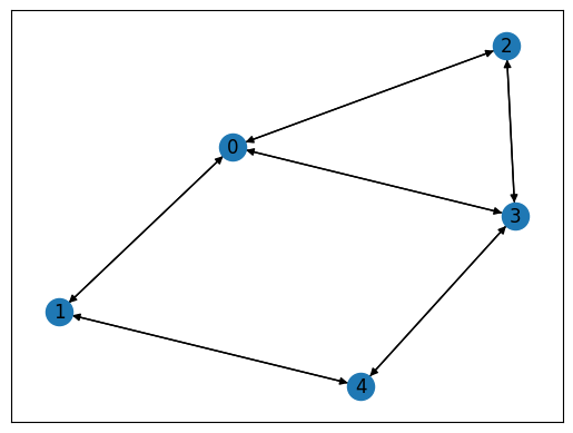
このグラフを図示すると、次のようになります。

import matplotlib.pyplot as plt

# Compute the layout
pos = nx.spring_layout(inst_G)

nx.draw_networkx(inst_G, pos=pos, with_labels=True)
plt.show()

JijSolverで解く

jijsolverを用いて、この問題を解いてみましょう。

import jijsolver

interpreter = jm.Interpreter(instance_data)
instance = interpreter.eval_problem(problem)
solution = jijsolver.solve(instance, time_limit_sec=1.0)

解の可視化

次のようにして、得られた結果を表示してみましょう。

import matplotlib.pyplot as plt
import numpy as np

df = solution.decision_variables
x_indices = df[df["value"]==1]["subscripts"].to_list()
# sort by time step
path = [index for index, _ in sorted(x_indices, key=lambda x: x[1])]
# append start point
path.append(path[0])    
# make the directed graph from paths
inst_DG = nx.DiGraph()
inst_DG.add_edges_from([(path[i], path[i+1]) for i in range(len(path)-1)])
# create the figure with two subplots
fig, (ax1, ax2) = plt.subplots(1, 2, figsize=(10, 5))
# draw the initial graph
nx.draw_networkx(inst_G, pos, with_labels=True, ax=ax1)
ax1.set_title('Initial Graph')
plt.axis('off')
ax1.set_frame_on(False) # Remove the frame from the first subplot
# draw the directed graph
nx.draw_networkx_nodes(inst_DG, pos)
nx.draw_networkx_edges(inst_DG, pos, arrows=True)
nx.draw_networkx_labels(inst_DG, pos)
plt.axis('off')
ax2.set_title('Hamiltonian Cycle Graph')
# show the graphs
plt.show()

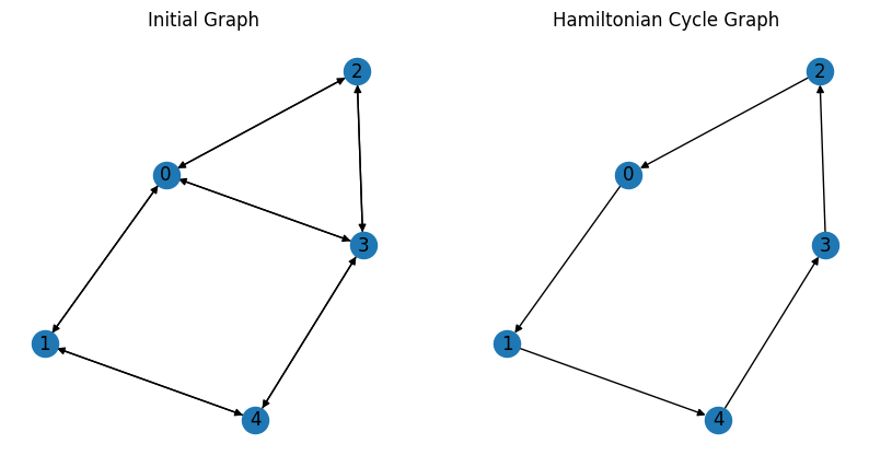
予想通り、ハミルトニアンサイクルを得ることができました。