多様性を含めたEコマースサイトのアイテムリスト最適化#
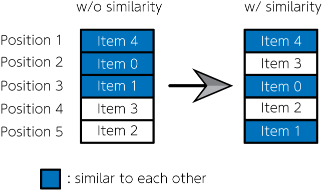
商品販売・宿泊施設予約・音楽や動画配信サイトのように、課金システムを持つEコマースサイトは、私たちにとって身近なものとなりました。これらのサイトを見ると、様々なアイテムが掲載されています。掲載されるアイテムをどのように決定するか、どのような配置で並べるかは、Eコマースサイトの売り上げに直結する重要な問題です。単純に売上数などの人気順で並べてしまうと、類似性の高いアイテムが連続して配置されることが多く、特定の趣味趣向に偏る可能性があります。そこでNishimura et al., 2019では、類似度の高い項目が隣り合って配置されることに対するペナルティなどを用い、項目リスト問題を二次割り当て問題として定式化しました。そしてそれを量子アニーリングで解き、アイテムの人気度と多様性を考慮したアイテムリストを作成するのに成功しました。今回はこの問題を題材にして、JijModelingによる数理モデル実装と、JijZeptSolverでの求解をしてみましょう。
数理モデル#
ウェブサイトのどの位置にどのアイテムを掲載するかを考えましょう。 掲載されるアイテムの集合を\(I\)、アイテムが掲載される位置の集合を\(J\)と定義します。 アイテム\(i\)を\(j\)番目の位置に配置するとき\(x_{i, j} = 1\)、それ以外の場合には\(x_{i, j} = 0\)となるようなバイナリ変数を用います。
各アイテムはどこか一箇所に掲載されなければならない#
一つの場所には一つのアイテムしか掲載できない#
目的関数#
アイテム\(i\)を\(j\)番目の位置に配置したときに予想される人気や売上を\(s_{ij}\)のように書きます。すると
が、最大化したいものです。 しかし上述したように、この目的関数だけでは同じ趣向のアイテムばかりが掲載されることになり、最適な配置とは考えられない解を得ます。 よって、目的関数に以下のような項を導入しましょう。
ここで\(f_{ii’}\)はアイテム\(i\)とアイテム\(i’\)の類似度を表します。 そして\(d_{jj’}\)は、\(j\)番目と\(j’\)番目の配置が隣り合うとき1、そうでないとき0となるような関数です。 これにより、隣り合う位置に類似度が大きいアイテムが並ぶような解は、目的関数の値が小さくなります。 以上の議論から、この最適化問題で最大化したい関数は
のように定式化されます。 第二項の係数\(w\)は、第二項の重みを調整するためのものです。
問題分割#
大きな問題の場合、実行可能解が求まらないことや、仮に求まったとしても最適解から遠い場合があります。 そこで、まずは(3)式を目的関数とした最適化問題を解きます。 その後、アイテムリストの中でも上位に表示されるアイテムに対し、(5)式を用いた最適化問題を解きます。 これにより、閲覧頻度の高い上位のアイテムを効果的に決定することができます。
実装しましょう#
ここからは、実際にJijModelingとJijZeptSolverを用いて、この問題を解くスクリプトを実装しましょう。
変数の定義#
以下のようにして、最適化に用いる変数を定義します。 まずは(3)式を目的関数とした場合の数理モデルの実装を考えましょう。
import jijmodeling as jm

# define variables
I = jm.Placeholder('I')
J = jm.Placeholder('J')
s = jm.Placeholder('s', ndim=2)
x = jm.BinaryVar('x', shape=(I, J))
i = jm.Element('i', belong_to=I)
j = jm.Element('j', belong_to=J)
Iはアイテムの集合、Jはアイテムを掲載する場所の集合、sは売り上げ予想を表す行列です。
xは最適化に用いるバイナリ変数、そしてi, jはそれぞれ数理モデルに用いる添字を表します。
数理モデルの実装#
続いて、(1), (2)式の制約と、(3)式の目的関数で表される数理モデルを実装しましょう。
# make problem
problem = jm.Problem('E-commerce', sense=jm.ProblemSense.MAXIMIZE)
# set constraint 1: onehot constraint for items
problem += jm.Constraint('onehot-items', jm.sum(j, x[i, j])==1, forall=i)
# set constraint 2: onehot constraint for position
problem += jm.Constraint('onehot-positions', jm.sum(i, x[i, j])==1, forall=j)
# set objective function 1: maximize the sales
problem += jm.sum([i, j], s[i, j]*x[i, j])
Problemで問題を作成します。
引数senseにProblemSense.MAXIMIZEを入力することで、目的関数を最大化する問題として実装することができます。
Constaintで2つの制約を追加します。
制約や目的関数の追加には、+=演算子を用います。
Jupyter Notebook上で、実装した数理モデルを確認することができます。
problem
インスタンス作成#
次に、インスタンスを作成します。
ここではアイテム数を10、そしてアイテムを掲載する場所の数も10とします。
また、売り上げ予想行列sはランダムとします。
import numpy as np

# set the number of items
inst_I = 10
inst_J = 10
inst_s = np.random.rand(inst_I, inst_J)
# set instance for similarity term
inst_f = np.random.rand(inst_I, inst_I)
triu = np.tri(inst_J, k=1) - np.tri(inst_J, k=0)
inst_d = triu + triu.T
instance_data = {'I': inst_I, 'J': inst_J, 's': inst_s, 'f': inst_f, 'd': inst_d}
JijZeptSolverで解く#
JijZeptSolverを用いて、先程実装した問題を解いてみましょう。
import jijzept_solver

interpreter = jm.Interpreter(instance_data)
instance = interpreter.eval_problem(problem)
solution = jijzept_solver.solve(instance, time_limit_sec=1.0)
解のチェック#
計算結果をチェックしてみましょう。
df = solution.decision_variables_df
x_indices = np.array(df[df["value"]==1]["subscripts"].to_list())
# initialize binary array
pre_binaries = np.zeros([inst_I, inst_J], dtype=int)
# input solution into array
pre_binaries[x_indices[:, 0], x_indices[:, 1]] = 1
# format solution for visualization
pre_zip_sort = sorted(zip(np.where(np.array(pre_binaries))[1], np.where(np.array(pre_binaries))[0]))
for pos, item in pre_zip_sort:
    print('{}: item {}'.format(pos, item))
# compute similarity for comparison later
A = np.dot(instance_data['f'], pre_binaries)
B = np.dot(pre_binaries, instance_data['d'])
AB = A * B
pre_similarity = np.sum(AB)
0: item 7
1: item 0
2: item 4
3: item 1
4: item 6
5: item 5
6: item 8
7: item 2
8: item 3
9: item 9
問題の分割: ペナルティ項と変数固定の活用#
先ほどは全ての変数に対して組合せ最適化問題を解きました。 次はさらに、上位のアイテムに対してアイテム類似度を考慮した目的関数(5)式で、最適化問題を解きましょう。 そのために新しく変数を定義します。
# set variables for sub-problem
fixed_IJ = jm.Placeholder('fixed_IJ', ndim=2)
f = jm.Placeholder('f', ndim=2)
d = jm.Placeholder('d', ndim=2)
k = jm.Element('k', belong_to=I)
l = jm.Element('l', belong_to=J)
fixed_ij = jm.Element('fixed_ij', belong_to=fixed_IJ)
fixed_IJは次の最適化問題では解かない、変数を固定する添字の集合を表します。
これは二次元配列として表現され、例えば\(x_{5, 6} = 1, x_{7, 8} =1\)のように固定する場合にはfixed_{IJ} = [[5, 6], [7, 8]]のようになります。
fはアイテム類似度を表す行列、dは配置が隣り合うかどうかを表す行列です。
k, l, fixed_ijは、新しい添字を定義しています。
次に、アイテムの類似度を最小化するための項を追加しましょう。
# set penalty term 2: minimize similarity
# problem += jm.CustomPenaltyTerm('similarity', jm.sum([i, j, k, l], f[i, k]*d[j, l]*x[i, j]*x[k, l]))
problem += jm.sum([i, j, k, l], f[i, k]*d[j, l]*x[i, j]*x[k, l])
ここではCustomPenaltyTermを用いて、アイテム類似度の項を表現しています。
これは、ゼロになる必要はないがなるべくゼロになってほしい、ソフト制約を表しています。
最後に、下位に表示されているアイテムに関しては変数を先ほどの最適化結果で固定し、上位のアイテムについてだけの最適化を行うようにしましょう。
# set fixed variables
problem += jm.Constraint('fix', x[fixed_ij[0], fixed_ij[1]]==1, forall=fixed_ij)
Constraintを用いることで、変数固定を自明な制約として記述することができます。
Jupyter Notebook上で、新たに追加された項などを表示してみましょう。
problem
数理モデルの実装が完了したところで、アイテム類似度と変数固定のためのインスタンスを作成しましょう。
# set instance for fixed variables
reopt_N = 5
item_indices = x_indices[:, 0]
position_indices = x_indices[:, 1]
fixed_indices = np.where(np.array(position_indices)>=reopt_N)
fixed_items = np.array(item_indices)[fixed_indices]
fixed_positions = np.array(position_indices)[fixed_indices]
instance_data['fixed_IJ'] = np.array([[x, y] for x, y in zip(fixed_items, fixed_positions)])
そして類似度に関するペナルティと変数固定を考慮した数理モデルを、JijZeptSolverで最適化計算しましょう。
interpreter = jm.Interpreter(instance_data)
instance = interpreter.eval_problem(problem)
solution = jijzept_solver.solve(instance, time_limit_sec=1.0)
再び、得られた解をチェックしてみましょう。
df = solution.decision_variables_df
x_indices = np.array(df[df["value"]==1]["subscripts"].to_list())
# initialize binary array
post_binaries = np.zeros([inst_I, inst_J], dtype=int)
# input solution into array
post_binaries[x_indices[:, 0], x_indices[:, 1]] = 1
# format solution for visualization
post_zip_sort= sorted(zip(np.where(np.array(post_binaries))[1], np.where(np.array(post_binaries))[0]))
for i, j in post_zip_sort:
    print('{}: item {}'.format(i, j))
# compute similarity for comparison later
A = np.dot(instance_data['f'], pre_binaries)
B = np.dot(post_binaries, instance_data['d'])
AB = A * B
post_similarity = np.sum(AB)
0: item 7
1: item 0
2: item 1
3: item 6
4: item 4
5: item 5
6: item 8
7: item 2
8: item 3
9: item 9
2つの結果を比較してみましょう。
items = ["Item {}".format(i) for i in np.where(pre_binaries==1)[0]]
pre_order = np.where(pre_binaries==1)[1]
post_order = np.where(post_binaries==1)[1]
グラフ描画のために、次のようなクラスを定義しましょう。
from typing import Optional
import matplotlib.pyplot as plt

class Slope:
    """Class for a slope chart"""
    def __init__(self,
        figsize: tuple[float, float] = (6,4),
        dpi: int = 150,
        layout: str = 'tight',
        show: bool =True,
        **kwagrs):

        self.fig = plt.figure(figsize=figsize, dpi=dpi, layout=layout, **kwagrs)
        self.show = show

        self._xstart: float = 0.2
        self._xend: float = 0.8
        self._suffix: str = ''
        self._highlight: dict = {}

    def __enter__(self):
        return(self)

    def __exit__(self, exc_type, exc_value, exc_traceback):
        plt.show() if self.show else None

    def highlight(self, add_highlight: dict) -> None:
        """Set highlight dict

        e.g.
            {'Group A': 'orange', 'Group B': 'blue'}

        """
        self._highlight.update(add_highlight)

    def config(self, xstart: float =0, xend: float =0, suffix: str ='') -> None:
        """Config some parameters

            Args:
                xstart (float): x start point, which can take 0.0〜1.0
                xend (float): x end point, which can take 0.0〜1.0
                suffix (str): Suffix for the numbers of chart e.g. '%'

            Return:
                None

        """
        self._xstart = xstart if xstart else self._xstart
        self._xend = xend if xend else self._xend
        self._suffix = suffix if suffix else self._suffix

    def plot(self, time0: list[float], time1: list[float],
             names: list[float], xticks: Optional[tuple[str,str]] = None,
             title: str ='', subtitle: str ='', ):
        """Plot a slope chart

        Args:
            time0 (list[float]): Values of start period
            time1 (list[float]): Values of end period
            names (list[str]): Names of each items
            xticks (tuple[str, str]): xticks, default to 'Before' and 'After'
            title (str): Title of the chart
            subtitle (str): Subtitle of the chart, it might be x labels

        Return:
            None

        """

        xticks = xticks if xticks else ('Before', 'After')

        xmin, xmax = 0, 4
        xstart = xmax * self._xstart
        xend = xmax * self._xend
        ymax = max(*time0, *time1)
        ymin = min(*time0, *time1)
        ytop = ymax * 1.2
        ybottom = ymin - (ymax * 0.2)
        yticks_position = ymin - (ymax * 0.1)

        text_args = {'verticalalignment':'center', 'fontdict':{'size':10}}

        for t0, t1, name in zip(time0, time1, names):
            color = self._highlight.get(name, 'gray') if self._highlight else None

            left_text = f'{name} {str(round(t0))}{self._suffix}'
            right_text = f'{str(round(t1))}{self._suffix}'

            plt.plot([xstart, xend], [t0, t1], lw=2, color=color, marker='o', markersize=5)
            plt.text(xstart-0.1, t0, left_text, horizontalalignment='right', **text_args)
            plt.text(xend+0.1, t1, right_text, horizontalalignment='left', **text_args)

        plt.xlim(xmin, xmax)
        plt.ylim(ytop, ybottom)

        plt.text(0, ytop, title, horizontalalignment='left', fontdict={'size':15})
        plt.text(0, ytop*0.95, subtitle, horizontalalignment='left', fontdict={'size':10})

        plt.text(xstart, yticks_position, xticks[0], horizontalalignment='center', **text_args)
        plt.text(xend, yticks_position, xticks[1], horizontalalignment='center', **text_args)
        plt.axis('off')


def slope(
    figsize=(6,4),
    dpi: int = 150,
    layout: str = 'tight',
    show: bool =True,
    **kwargs
    ):
    """Context manager for a slope chart"""

    slp = Slope(figsize=figsize, dpi=dpi, layout=layout, show=show, **kwargs)

    return slp
最後に、比較のためのグラフを表示しましょう。
pre_string = "Similarity: {:.2g}".format(pre_similarity)
post_string = "Similarity: {:.2g}".format(post_similarity)
with slope() as slp:
    slp.plot(pre_order, post_order, items, (pre_string, post_string))
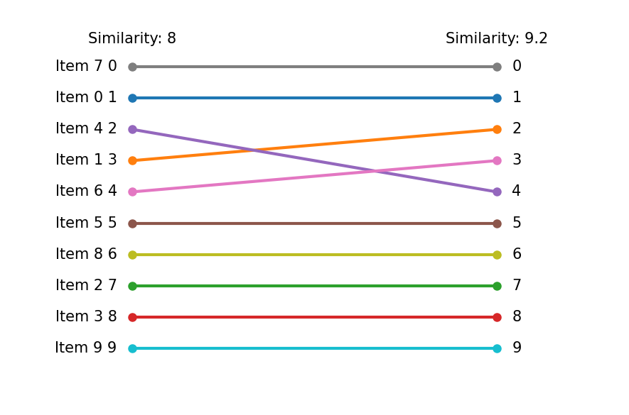
最初の最適化結果と比較すると、下位部分は変数固定により変化はありません。 しかし、上位部分は類似度を考慮したことで、順番に変動が見られます。