最大次数制約を持つ最小スパニングツリー問題

ここではJijSolverとJijModelingを用いて、最大次数制約を持つ最小スパニングツリー問題を解く方法を説明します。 この問題は、Lucas, 2014, “Ising formulations of many NP problems” 8.1. Minimal Spanning Tree with a Maximal Degree Constraint で触れられています。

最大次数制約を持つ最小スパニングツリー問題とは

最小スパニングツリー問題は、次のように定義されます。 各辺\((uv) \in E\)がそれぞれコスト\(c_{uv}\)を持つような、無向グラフ\(G=(V, E)\)が与えられたとします。 全ての頂点を含むようなツリーである、スパニングツリー \(T \subseteq G\)を構築することを考えます。 もし\(T\)が存在するとき、そのコスト

\[ c(T) = \sum_{(uv) \in E_T} c_{uv} \]

を最小化することを考えるのが、この最小スパニングツリー問題です。 そしてここに、\(T\)に含まれる頂点の次数が\(\Delta\)以下でなければならないという、最大次数制約を加えます。

例題

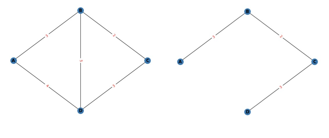
簡単のため、ここでは次のような単純なグラフを見てみましょう。 左グラフにおいて、最大次数が3で制限されるような、最小スパニングツリーを求めてみましょう。 この問題に対する答えは、右のグラフのようになります。 このツリーの重みの総和は8で最小です。 そして最大次数制約も満たされていることがわかります。

数理モデル

辺\(e=(uv)\)が最小スパニングツリー\(T\)に含まれるとき1、そうでないとき0となるようなバイナリ変数\(x_{uv}\)を導入します。

制約 1: 各頂点は最大で\(\Delta\)まで辺を持つことができる

グラフにおけるどの頂点の次数も、\(\Delta\)を超えることはできません。 ツリーでは少なくとも1つの辺を持たなければならないため、各頂点の次数に下界を考える必要があります。

\[ \quad 1 \leq \sum_{(uv),(vu) \in E} x_{uv} \leq \Delta \quad \forall u \in V. \]

\(x_{uv}, x_{vu}\)についての総和であることに注意が必要です。

制約 2: ツリーは全ての頂点を含めなければならない

選択された辺は、全ての頂点を含めるような木を形成しなければなりません。 もし\(T\)の辺の合計が\(|V|-1\)より小さいならば、\(T\)は全ての辺を含めることができません。 そして\(T\)の辺の合計が\(|V|-1\)より大きければ、\(T\)はツリーではなくなります (この場合、グラフにループが存在することになります。)

\[ \quad \sum_{(uv) \in E} x_{uv} = |V|-1. \]

制約 3: 切断制約

この制約により、解のグラフがバラバラでなく接続されており、非巡回グラフとなることを保証します。

\[ \quad \sum_{(uv) \in E(S)} x_{uv} \leq |S| - 1 \quad \forall S \subset G, \]

ここで\(S\)はグラフ\(G\)の部分グラフ、そして\(E(S)\)は\(S\)内に含まれる辺の集合です。

目的関数

\(T\)の重みの総和を最小化する目的関数を設定します。

\[ \quad \min \sum_{uv \in E} c_{uv}x_{uv}. \]

JijModelingによるモデル化

次に、JijModelingを用いて数理モデルを実装しましょう。 最初に、上述の数理モデルに必要な変数を定義します。

import jijmodeling as jm

#define variables
V = jm.Placeholder('V')  # number of vertices
E = jm.Placeholder('E', ndim=2)  # set of edges
num_E = E.shape[0]
C = jm.Placeholder('C', ndim=2)  # cost between each vertex
D = jm.Placeholder('D')  # number of degrees
S = jm.Placeholder('S', ndim=3)  # list of set of subgraph edges
num_S = S.shape[0]
S_nodes = jm.Placeholder('S_nodes', ndim=1)  # list of number of subgraphs vertices

x = jm.BinaryVar('x', shape=(num_E,))

v = jm.Element('v', V)  # subscripts for verteces
e = jm.Element('e', num_E)  # subscripts for edges
i_s = jm.Element('i_s', num_S)
e_s = jm.Element('e_s', S[i_s].shape[0])  # subscripts of edges in S

制約と目的関数を実装しましょう。

problem = jm.Problem("minimum spanning tree with a maximum degree constraint")
problem += jm.Constraint('const1-1', jm.sum((e, (E[e][0]==v)|(E[e][1]==v)), x[e]) >= 1, forall=v)
problem += jm.Constraint('const1-2', jm.sum((e, (E[e][0]==v)|(E[e][1]==v)), x[e]) <= D, forall=v)
problem += jm.Constraint('const2', x[:].sum() == V-1)
problem += jm.Constraint('const3',jm.sum(e_s, x[e_s]) <= S_nodes[i_s] - 1, forall = i_s)
problem += jm.sum(e, C[E[e][0]][E[e][1]]*x[e])

Jupyter Notebook上で、実装した数理モデルを表示してみましょう。

problem 

\[\begin{split}\begin{array}{cccc}\text{Problem:} & \text{minimum spanning tree with a maximum degree constraint} & & \\& & \min \quad \displaystyle \sum_{e = 0}^{\mathrm{len}\left(E, 0\right) - 1} C_{E_{e, 0}, E_{e, 1}} \cdot x_{e} & \\\text{{s.t.}} & & & \\ & \text{const1-1} & \displaystyle \sum_{\substack{e = 0\\E_{e, 0} = v \lor E_{e, 1} = v}}^{\mathrm{len}\left(E, 0\right) - 1} x_{e} \geq 1 & \forall v \in \left\{0,\ldots,V - 1\right\} \\ & \text{const1-2} & \displaystyle \sum_{\substack{e = 0\\E_{e, 0} = v \lor E_{e, 1} = v}}^{\mathrm{len}\left(E, 0\right) - 1} x_{e} \leq D & \forall v \in \left\{0,\ldots,V - 1\right\} \\ & \text{const2} & \displaystyle \sum_{\ast_{0} = 0}^{\mathrm{len}\left(E, 0\right) - 1} x_{\ast_{0}} = V - 1 & \\ & \text{const3} & \displaystyle \sum_{e_s = 0}^{\mathrm{len}\left(S_{i_s}, 0\right) - 1} x_{e_s} \leq S_nodes_{i_s} - 1 & \forall i_s \in \left\{0,\ldots,\mathrm{len}\left(S, 0\right) - 1\right\} \\\text{{where}} & & & \\& x & 1\text{-dim binary variable}\\\end{array}\end{split}\]

インスタンスの準備

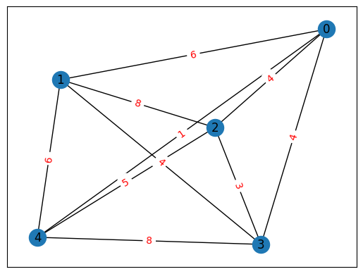
NetworkXを用いて、グラフを準備しましょう。 例として、ランダムな完全グラフ (全ての頂点がお互いに接続されているようなグラフ) を作成しましょう。

import itertools
import networkx as nx
import numpy as np

np.random.seed(seed=0)

# set the number of vertices
inst_V = 5
# set the number of degree
inst_D = 2

# set the probability of rewiring edges
p_rewire = 0.2
# set the number of nearest neighbors
k_neighbors = 4
# create a connected graph
inst_G = nx.connected_watts_strogatz_graph(inst_V, k_neighbors, p_rewire)
# add random costs to the edges
for u, v in inst_G.edges():
    inst_G[u][v]['weight'] = np.random.randint(1, 10)

# create a 2D array for the costs
inst_C = np.zeros((inst_V, inst_V))
for u, v in inst_G.edges():
    inst_C[u][v] = inst_G[u][v]['weight']
    inst_C[v][u] = inst_G[u][v]['weight']
# set diagonal elements to infinity
np.fill_diagonal(inst_C, np.inf)

# get information of edges
inst_E = [list(edge) for edge in inst_G.edges]

# get subgraphs and their edges
sub_nodes = []
sub_edges = []
# get connected subgraphs that have at least 2 nodes and have less nodes than the original graph
for num_nodes in range(2, inst_G.number_of_nodes()):
    for comb in (inst_G.subgraph(selected_nodes) for selected_nodes in itertools.combinations(inst_G, num_nodes)):
        if nx.is_connected(comb):
            sub_edges.append(comb.edges)
            sub_nodes.append(comb.nodes)
inst_S = [list(edgeview) for edgeview in sub_edges]
inst_S = [[list(t) for t in inner_list] for inner_list in inst_S]  # convert tuples into lists
# get the number of vertices in each subgraph
inst_S_nodes = [len(x) for x in sub_nodes]

instance_data = {'V': inst_V, 'D': inst_D, 'E': inst_E, 'C': inst_C, 'S': inst_S, 'S_nodes': inst_S_nodes}

ここで作られたグラフを表示してみます。

import matplotlib.pyplot as plt

pos = nx.spring_layout(inst_G)
nx.draw_networkx(inst_G, pos, with_labels=True)
edge_labels = nx.get_edge_attributes(inst_G, 'weight')
nx.draw_networkx_edge_labels(inst_G, pos, edge_labels=edge_labels, font_color='red')

plt.show()

Solve by JijSolver

この問題をjijsolverを用いて解きましょう。

import jijsolver

interpreter = jm.Interpreter(instance_data)
instance = interpreter.eval_problem(problem)
solution = jijsolver.solve(instance, time_limit_sec=1.0)

/opt/hostedtoolcache/Python/3.9.22/x64/lib/python3.9/site-packages/jijsolver/solver.py:196: UserWarning: Return empty `Samples` since an error occurred in process #1 during the calculation: Model was infeasible
  warnings.warn(

解の可視化

得られた解を可視化してみましょう。

# get the indices of x == 1
df = solution.decision_variables
x_indices = df[df["value"]==1]["subscripts"].to_list()# set edge color list (x==1: black, x==0: white)
inst_E = np.array(inst_E)
mask = inst_E[:, 0] > inst_E[:, 1]
inst_E[mask] = inst_E[mask][: , : :-1]
edge_colors = np.where(np.isin(np.arange(len(inst_E)), x_indices), 'black', 'white').tolist()
# draw figure
plt.subplot(121)
plt.axis('off')
nx.draw(inst_G, pos, with_labels=True, font_weight='bold')
nx.draw_networkx_edge_labels(inst_G, pos, edge_labels=edge_labels, font_color='red')
plt.subplot(122)
plt.axis('off')
inst_H = inst_G.copy()
for i in range(len(inst_H.edges)):
    if edge_colors[i] == 'white':
        inst_H.remove_edge(*list(inst_G.edges)[i])
nx.draw(inst_H, pos, with_labels=True, font_weight='bold')
nx.draw_networkx_edge_labels(inst_H, pos, edge_labels=nx.get_edge_attributes(inst_H, 'weight'), font_color='red')

{(0, 4): Text(0.0101088538277197, 0.09041778994639327, '1'),
 (0, 2): Text(0.5036471505168673, 0.5704329609042784, '4'),
 (1, 3): Text(-0.10706160643656223, -0.1608507508506712, '4'),
 (2, 3): Text(0.32227220970036413, -0.37000178998260946, '3')}

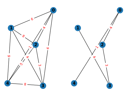
期待通り、最大次数制約を満たす最小スパニングツリーを得ることができました。
ここで紹介した問題の高度な発展として、シュタイナーツリー問題というものがあります。 この問題は次のようなものです。 辺のコスト\(c_{uv}\)が与えられたとき、頂点の部分集合\(U \subset V\)に対して最小スパニングツリーを考えます。 ここで\(U\)に含まれないノードの使い方は、自由とします。 この問題を解くには、最小スパニングツリー問題と同じハミルトニアンを用いることができますが、頂点\(v\)が\(U\)に含まれるかどうかを表す追加のバイナリ変数\(y_v\)を用いる必要があります。